
Part 1 : AR, MA, ARMA (Stationary Model)
Part 2 : ARIMA, Seasonal ARIMA (Non-Stationary Model) <- this post
In my previous post, I have explained AR, MA, and ARMA under stationary condition.
In this post, I proceed to non-stationary models, ARIMA.
Many of real cases (stock price, sales revenue, etc) are non-stationary time series or mixed ones. However it’s also important to understand the idea of stationary model, because the idea of non-stationarity is based on the stationary model.
5. Non-Stationary Time Series
The idea of non-stationary model is :
- Make the series of differences
.
- Consider stationarity for these difference series.
If the difference series is stationary model given as ARMA(p, q), we can estimate the model of differences with methods in previous post, and we can then take the original 
In general, ARIMA(p, d, q) is given by the definition as : the series of d-th order difference is ARMA(p, q).
As I have described in my previous post, all MA model is stationary. Therefore we can focus on AR part for considering non-stationary model.
Even though there exists a little difference between parameters 

Let’s see the following example (curve) for different 
Sample of 
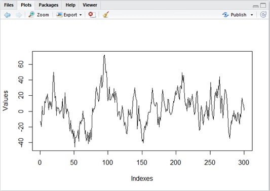
Sample of 
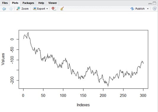
Sample of 
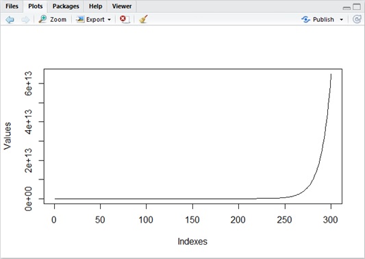
Unlike the stationary process, non-stationary process diverges in general. (See above in 
Thus we cannot apply the same mathematical methods with stationary process for non-stationary one. Under the condition of non-stationarity, we cannot also use t-distribution (which is often used as statistical distribution) for estimation.
Now let’s see how we can estimate non-stationary model.
First we consider the following AR expression (1). (See my previous post for 

In this model, the following equation (2) is called “characteristic equation” :

It’s known that this equation follows the properties, such as :
- If all the absolute values of roots of equation (2) are larger than 1, (1) is stationary.
- If
is a root of
multiplicity (i.e, the characteristic equation (2) has the term
in the factor) and the absolute values of other roots are all larger than 1, the series of d-th order difference of (1) is stationary.
Especially, if (2) has only one unit root (d = 1), the series ofof (1) will become stationary.
This model is called unit root process.
Note : Later in this post, I’ll show you why this holds.
Now let’s start using the simple case of AR(1), which has the following equation.

In this case, we can find :
- It’s stationary if
.
- It will be unit root process if
.
If
In general, you can repeat this process for series 
Our next concern is : how to know whether it’s unit root process, when time series 
6. Estimate Model and Forecast in ARIMA
Under the condition of unit root process, we cannot use t-distribution for estimation, because it is not stationary. Instead of that, we can use Dickey-Fuller test to distinguish whether model is unit root process.
Here (in this post) I don’t discuss details about Dickey-Fuller test, but the outline is below.
In order to simplify, I assume 
- Consider the following continuous stochastic process
, where
is the size of given time series data and
is standard deviation of
.
Intuitively, this will mapinto
on the range
separated by the segment of each spans
.
- When
in stochastic distribution. (See “Donsker’s theorem“.)
Note that Wiener processhas properties
and
.
Thenis
and
is
.
- It’s known that the following convergence with Wiener process holds, when
whereis the least-squares estimator of
, and
is the standard error of least-squares estimator


This value (LHS of equation (3)) belongs to a specific distribution known as the Dickey–Fuller table, and you can then examine Dickey–Fuller test for finding whether it’s unit root process.
On contrary, it is known that the following value (t statistics) is on t-distribution table when
Note : This describes Dickey-Fuller t-test for your understanding, but there also exists another Dickey-Fuller ρ-test.
There exists an extension of Dickey–Fuller test to AR(p), called Augmented Dickey–Fuller (ADF) test, and ADF test is used in practice.
Here I don’t describe details about this test (ADF), but with programming in R, you can simply use adf.test() (in tseries package) for running ADF test.
Now, let’s estimate the following time series data with linear positive trend in R script.
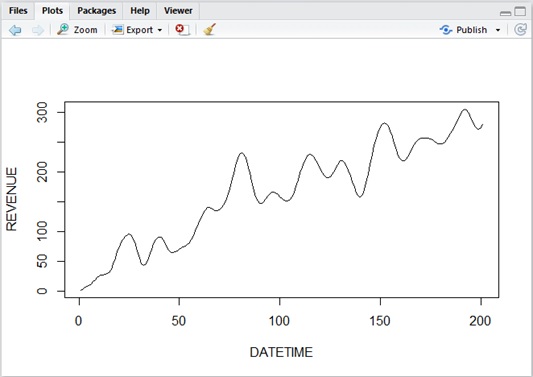
Same like the stationary model (see my previous post), you can simply use auto.arima() for identifying model and estimating parameters, also for ARIMA. (See below.)
You don’t need to follow previous steps in your programming code.
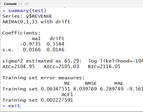
library(forecast)# read datay <- read.table( "C:\Demo\revenue_sample.txt", col.names = c("DATETIME", "REVENUE"), header = TRUE, quote = """, fileEncoding="UTF-8", stringsAsFactors = FALSE)# analyzetest = auto.arima(y$REVENUE)summary(test)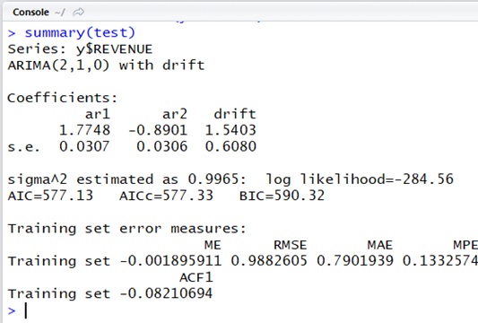
Here the obtained model of 
The result “drift” (see the output above) means the trend of

and

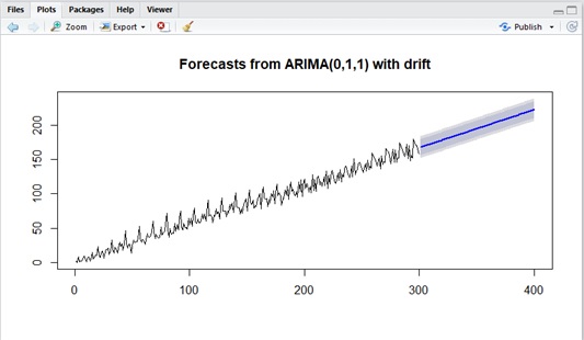
The following is the forecasting for the obtained model. (See below.)
Please compare the following predicted plotting (non-stationary result) with the one in my previous post (stationary result).
Unlike stationary model, the predicted mean (conditional mean) will not converge to the mean of model (it will always move by drift) and the predicted variance will also grow more and more.
...# analyzetest = auto.arima(y$REVENUE)summary(test)# predictpred <- forecast( test, level=c(0.85,0.95), h=50)plot(pred)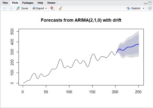
In auto.arima(), it will repeatedly test the difference 
In the next topic, I will discuss how these seasonality can be solved in ARIMA.
7. Backshift Notation
Before I discuss seasonal ARIMA, let me introduce convenient notation called “backshift notation”.
With this notation we denote 


Same like this, 

With this notation, the following transition holds.

With this notation, we can easily treat the time series differences by such like arithmetic operations.
For example, 


By repeating this operation, you can denote p-th order difference by 
With this notation, ARIMA(1,1,0) is denoted by the following equation, where 


As you can see above, this notation clarifies the structure of model, because 


Thus, when you want to denote ARIMA(1,d,0), you can easily get by the following representation.

Now I rewrite the previous equation (1) with backshift notation as follows.


As you can see above, LHS (left-hand-side) in the last expression is the same format with expression (2).
If (2) can be represented by 


As you saw above, you can easily get the previous consequence with backshift notation.
8. Seasonal ARIMA (SARIMA)
With backshift notation, you can easily understand seasonal ARIMA model.
First, I’ll show you the basic concept using simple AR(1) model with no difference d.
Suppose, the sales revenue is so much affected by the revenue of the same month a year ago (12 months ago).
Then this relation can be written by the following expression with backshift notation. (For simplicity, I skipped the constant value

Note :
means the seasonal part of
Suppose the revenue is also affected by the revenue from a month ago.
Then the mixed model will be represented as follows. This model is denoted by 

What does this model mean ? (Why it’s multiplied ?)
By transforming this representation, you will get the following :

As you can see above, 


Therefore this expression means “AR(1) model for the effect of one month ago, in which the effect of 12 months ago is eliminated”.
This is also written by the following representation. As you can see, it’s vice versa.

I have showed the above sample with no differences so far, but when it has the difference 
For example, 

In this expression :
is AR(1) of seasonal part.
is the difference of seasonal part.
Note : If you have MA(1), you can write on RHS as follows. (In this post, I don’t discuss about MA part in seasonal ARIMA.)

9. Find Seasonality
When I transform the equation of

Suppose, we don’t know the seasonality for given time series data. Then we must estimate with all possible difference (lags) and coefficients 
It will be time-consuming to search all possible lags. Please imagine if we have seasonality with seasonal lag = 365.
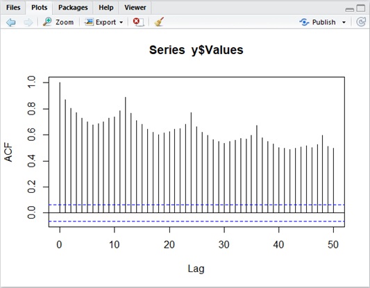
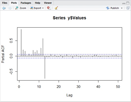
The following is ACF and PACF for 
As you can see in the following result, it has the spike at lags in seasonal part. Thus ACF and PACF can also be used in order to identify a seasonal model.
Autocorrelation (ACF) sample
Partial Autocorrelation (PACF) sample
Let’s see the brief example in R.
Now I’ll start to estimate the model and forecast with the obtained model as usual.
library(forecast)# read datay <- read.table( "C:\Demo\seasonal_sample.txt", col.names = c("DATETIME", "REVENUE"), header = TRUE, fileEncoding="UTF-8", stringsAsFactors = FALSE)# analyzetest <- auto.arima(y$REVENUE)summary(test)# predict and plotpred <- forecast( test, level=c(0.85,0.95), h=100)plot(pred)As I mentioned above, auto.arima() doesn’t test all possible lags.
Eventually I’ll get the result without seasonality (the result is ARIMA(0,1,1) with drift) as follows and the forecast plotting will become unexpected one.
Suppose we test with ACF/PACF and know that this dataset has possible seasonality with lag 12 (for instance, 12 months).
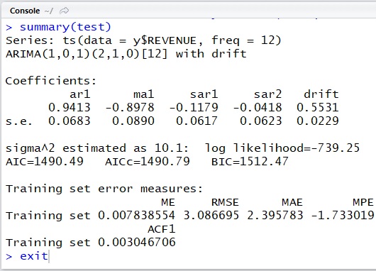
Now we can fix the previous R script to use this known seasonality as follows. (Here I have changed the code in bold fonts.)
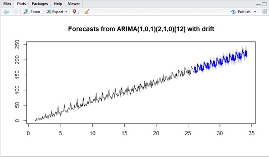
library(forecast)# read datay <- read.table( "C:\Demo\seasonal_sample.txt", col.names = c("DATETIME", "REVENUE"), header = TRUE, fileEncoding="UTF-8", stringsAsFactors = FALSE)# analyze with seasonal s=12test <- auto.arima(ts(data=y$REVENUE, freq=12))summary(test)# predict and plotpred <- forecast( test, level=c(0.85,0.95), h=100)plot(pred)As you can see below, now we can get the desirable result with seasonal ARIMA.
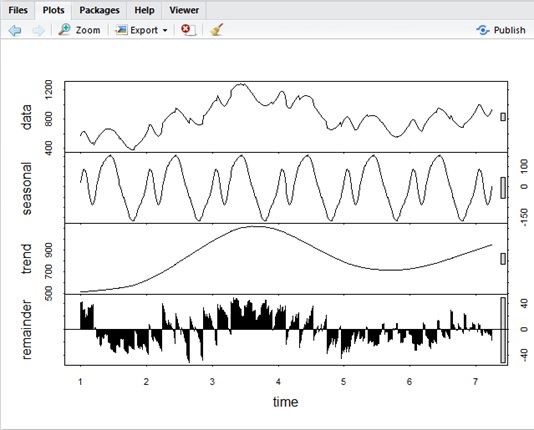
ARIMA doesn’t include the decomposition idea, but it’s sometimes useful to decompose and get properties (drift, seasonality) for time series data beforehand.
For instance, the following original data (“data” section in the following curves) is decomposed by stl() function in R as follows.
Categories: Uncategorized

this is abuot how to measured frequencies on microwaves on the radio system by megahertz and gigahertz the last diagram above show as the freguencies and the mega mesaurement is this µ .
LikeLike