
(You can download this example from here .)
In this post, I’ll introduce NVIDIA TensorRT inferencing for developers (data scientists) on Microsoft Azure.
Using Data Science Virtual Machine (DSVM) or NVIDIA GPU-optimized VMI on Azure, GPU drivers and other software (conda, etc) has already been installed without cumbersome settings.Azure Data Science Virtual Machine (DSVM) also includes TensorRT runtime (see here) and you can also soon start without setting up TensorRT software.
[Updated] Currently, TensorRT runtime is not included in Azure DSVM (Data Science Virtual Machine). I will then install TensorRT in DSVM as follows.
In this example, I’ll show you how to optimize models in TensorFlow by using TensorRT for ONNX.
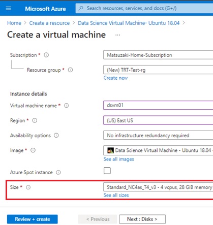
For running this example, here I use “Data Science Virtual Machine- Ubuntu 18.04” (DSVM) on Standard NC4as T4 v3 virtual machine (which has a single NVIDIA Tesla T4 GPU) in Azure.

When you manually setup software in Ubuntu virtual machine (without DSVM), see here.
Note : TensorRT is also packaged within Triton Inference Server container. To run Triton Inference Server on Azure, you can use Azure Machine Learning no-code deployment. (See here.)
You can use a variety of containers in NVIDIA GPU Cloud (NGC) with Microsoft Azure. (See here.)
Setup Conda Environment
Conda is already installed and setup on DSVM (data science virtual machine) in Azure.
In this example, we use TensorFlow 1.x pre-trained model and I then need Python version 3.6. (You cannot use Python 3.8 or later for running TensorFlow 1.x.)
By running conda command as follows, create new conda environment with Python 3.6 and the required packages.
# Create new conda environmentconda create -n myenv -y Python=3.6# Activate conda environmentconda activate myenv# Install required packages in this environmentconda install -c conda-forge numpy protobuf==3.16.0 libprotobuf=3.16.0conda install -c conda-forge onnxpip install tensorflow-gpu==1.15.5pip install tf2onnx==1.8.2conda install -c conda-forge matplotlibconda install -c conda-forge pycudaconda install -c anaconda pillowNote : Here we install ONNX runtime and related packages, because we will convert TensorFlow model to ONNX format later.
In this conda environment, we also set up jupyter notebook as follows.
# Install jupyter notebookpip install notebook# Install notebook integration for condaconda install nb_condaInstall TensorRT
As I have mentioned above, here we use data science virtual machine (DSVM) in Azure and CUDA is then already setup in this machine.
Before installing TensorRT, check the installed CUDA version, and then download the corresponding TensorRT installer. (You can see CUDA version by “apt list --installed” command.)
In this example, I assume CUDA version 11.3 and I then download the corresponding TensorRT 8.0 local repo file (nv-tensorrt-repo-ubuntu1804-cuda11.3-trt8.0.1.6-ga-20210626_1-1_amd64.deb).
After you have downloaded installation assets, see installation guide and install TensortRT in operating system (Ubuntu 18.04).
os="ubuntu1804"tag="cuda11.3-trt8.0.1.6-ga-20210626"sudo dpkg -i nv-tensorrt-repo-${os}-${tag}_1-1_amd64.debsudo apt-key add /var/nv-tensorrt-repo-${os}-${tag}/7fa2af80.pubsudo apt-get update# Install TensorRTsudo apt-get install tensorrt# Install when using TensorRT with Python 3sudo apt-get install python3-libnvinfer-devIn each conda environments to use TensorRT, you should manually install the TensorRT pip wheel as follows.
conda activate myenvpip install --upgrade setuptools pippip install nvidia-pyindexpip install nvidia-tensorrtRun Notebook
Start Jupyter notebook in your conda environment.
This will show the access url in console, such as http://localhost:8888/tree?token=xxxxxxxxxx.
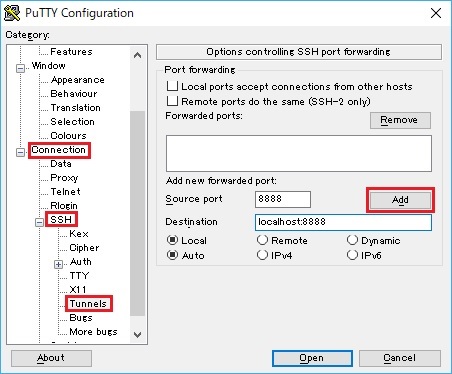
conda activate myenvjupyter notebookLaunch your terminal client (such as, PuTTY, etc), and connect to this machine by setting SSH tunnel (port forwarding) to access this notebook URL.
For instance, the following is the SSH tunnel setting on PuTTY terminal client in Windows. (In Mac OS, you can use ssh with -L option.)
Now you can run your code in Notebook on your browser.
Run Inference on TensorFlow (Without TensorRT)
First let’s start to run our example on standard TensorFlow without TensorRT inferencing. (You can download this example from here.)
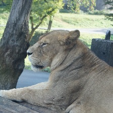
In this example, we run the inference for classification with pre-trained TensorFlow ResNet50 model (which is trained by ImageNet).
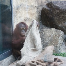
Here I’ll try to classify the following 3 photos (which I took at zoological park in Japan).
import matplotlib.image as mpimgimport matplotlib.pyplot as pltimport numpy as npimg = mpimg.imread('./tiger224x224.jpg')plt.imshow(np.array(img))plt.show()img = mpimg.imread('./lion224x224.jpg')plt.imshow(np.array(img))plt.show()img = mpimg.imread('./orangutan224x224.jpg')plt.imshow(np.array(img))plt.show()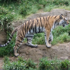
Before running classification, we convert the original images (3 photos) to fit the inputs in classification model.
The preprocessed images are included in the following image1, image2, and image3. (We will use these preprocessed images for classification.)
import tensorflow as tf## Create transformation graph#in_images = tf.placeholder(tf.string, name='in_images')decoded_input = tf.image.decode_jpeg(in_images, channels=3)float_input = tf.cast(decoded_input, dtype=tf.float32)# (224, 224, 3) -> (n, 224, 224, 3)rgb_input = tf.expand_dims( float_input, axis=0)# For VGG preprocess, reduce means and convert to BGRslice_red = tf.slice( rgb_input, [0, 0, 0, 0], [1, 224, 224, 1])slice_green = tf.slice( rgb_input, [0, 0, 0, 1], [1, 224, 224, 1])slice_blue = tf.slice( rgb_input, [0, 0, 0, 2], [1, 224, 224, 1])sub_red = tf.subtract(slice_red, 123.68)sub_green = tf.subtract(slice_green, 116.779)sub_blue = tf.subtract(slice_blue, 103.939)transferred_input = tf.concat( [sub_blue, sub_green, sub_red], 3)## Transform sample images#with tf.Session() as s1: with open('./tiger224x224.jpg', 'rb') as f:data1 = f.read()feed_dict = { in_images: data1}imglist1 = s1.run([transferred_input], feed_dict=feed_dict)image1 = imglist1[0] with open('./lion224x224.jpg', 'rb') as f:data2 = f.read()feed_dict = { in_images: data2}imglist2 = s1.run([transferred_input], feed_dict=feed_dict)image2 = imglist2[0] with open('./orangutan224x224.jpg', 'rb') as f:data3 = f.read()feed_dict = { in_images: data3}imglist3 = s1.run([transferred_input], feed_dict=feed_dict)image3 = imglist3[0]Now let’s run inference with original TensorFlow 1.x model on machine with a single NVIDIA Tesla T4 GPU (4 vcpus, 28 GiB memory).
See the results of how long does it take to inference.
import time## Load pre-trained classifier (ResNet 50)#classifier_model_file = './resnetV150_frozen.pb'classifier_graph_def = tf.GraphDef()with tf.gfile.Open(classifier_model_file, 'rb') as f: data = f.read() classifier_graph_def.ParseFromString(data)tf.import_graph_def( classifier_graph_def, name='classifier_graph')input_tf_tensor = tf.get_default_graph().get_tensor_by_name( 'classifier_graph/input:0')output_tf_tensor = tf.get_default_graph().get_tensor_by_name( 'classifier_graph/resnet_v1_50/predictions/Reshape_1:0')## Run inference#with open('./imagenet_classes.txt', 'rb') as f: labeltext = f.read() classes_entries = labeltext.splitlines()with tf.Session() as s2: # # predict image1 (tiger) # feed_dict = {input_tf_tensor: image1 } start_time = time.process_time() result = s2.run([output_tf_tensor], feed_dict=feed_dict) stop_time = time.process_time() # list -> 1 x n ndarray : feature's format is [[1.16643378e-06 3.12126781e-06 3.39836406e-05 ... ]] nd_result = result[0] # remove row's dimension onedim_result = nd_result[0,] # set column index to array of possibilities indexed_result = enumerate(onedim_result) # sort with possibilities sorted_result = sorted(indexed_result, key=lambda x: x[1], reverse=True) # get the names of top 5 possibilities print('********************') for top in sorted_result[:5]:print(classes_entries[top[0]], 'confidence:', top[1]) print('{:.2f} milliseconds'.format((stop_time-start_time)*1000)) # # predict image2 (lion) # feed_dict = {input_tf_tensor: image2 } start_time = time.process_time() result = s2.run([output_tf_tensor], feed_dict=feed_dict) stop_time = time.process_time() # list -> 1 x n ndarray : feature's format is [[1.16643378e-06 3.12126781e-06 3.39836406e-05 ... ]] nd_result = result[0] # remove row's dimension onedim_result = nd_result[0,] # set column index to array of possibilities indexed_result = enumerate(onedim_result) # sort with possibilities sorted_result = sorted(indexed_result, key=lambda x: x[1], reverse=True) # get the names of top 5 possibilities print('********************') for top in sorted_result[:5]:print(classes_entries[top[0]], 'confidence:', top[1]) print('{:.2f} milliseconds'.format((stop_time-start_time)*1000)) # # predict image3 (orangutan) # feed_dict = {input_tf_tensor: image3 } start_time = time.process_time() result = s2.run([output_tf_tensor], feed_dict=feed_dict) stop_time = time.process_time() # list -> 1 x n ndarray : feature's format is [[1.16643378e-06 3.12126781e-06 3.39836406e-05 ... ]] nd_result = result[0] # remove row's dimension onedim_result = nd_result[0,] # set column index to array of possibilities indexed_result = enumerate(onedim_result) # sort with possibilities sorted_result = sorted(indexed_result, key=lambda x: x[1], reverse=True) # get the names of top 5 possibilities print('********************') for top in sorted_result[:5]:print(classes_entries[top[0]], 'confidence:', top[1]) print('{:.2f} milliseconds'.format((stop_time-start_time)*1000))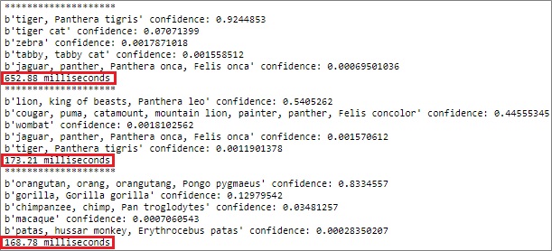
Run Inference with TensorRT
Next we run the same inference with TensorRT.
To use TensorRT optimizer for TensorFlow models, the only thing you should do is to convert models to ONNX format and use TensorRT with ONNX parser.
In this example, I’ll show you how to execute this workflow for the same TensorFlow model.
First, let’s convert TensorFlow model to ONNX format.
python3 -m tf2onnx.convert --input ./resnetV150_frozen.pb --inputs input:0 --outputs resnet_v1_50/predictions/Reshape_1:0 --output resnetV150_frozen.onnxNow let’s run inference with TensorRT for this ONNX model. (See the following code.)
This workflow for TensorRT inferencing is :
- Load ONNX model
- Create (Build) TensorRT engine using ONNX
- Serialize this engine into a file (.plan file)
- Load this engine (.plan file) on GPU device context
- Run inference with this loaded engine
import tensorrt as trtimport pycuda.driver as cudaimport tensorrt as trtimport timebatch_size = 1###### Load ONNX with TensorRT ONNX Parser,# Create an Engine,# and Serialize into a .plan file#####batch_size = 1TRT_LOGGER = trt.Logger(trt.Logger.WARNING)with trt.Builder(TRT_LOGGER) as builder, \ builder.create_network(1) as network, \ builder.create_builder_config() as config, \ trt.OnnxParser(network, TRT_LOGGER) as parser: config.max_workspace_size = (256 << 20) # Load ONNX with open("./resnetV150_frozen.onnx", 'rb') as model:parser.parse(model.read()) # Create engine network.get_input(0).shape = [batch_size , 224, 224, 3] engine = builder.build_engine(network, config) # Serialize engine in .plan file buf = engine.serialize() with open("./resnetV150_frozen.plan", 'wb') as f:f.write(buf)###### Make device context#####cuda.init()device = cuda.Device(0) # GPU id 0device_ctx = device.make_context()###### Load Engine and Define Inferencing Function###### Create page-locked memory buffers (which won't be swapped to disk)h_input_1 = cuda.pagelocked_empty(batch_size * trt.volume((1, 224, 224, 3)), dtype=trt.nptype(trt.float32))h_output = cuda.pagelocked_empty(batch_size * trt.volume((1, 1000)), dtype=trt.nptype(trt.float32))# Allocate device memoryd_input_1 = cuda.mem_alloc(h_input_1.nbytes)d_output = cuda.mem_alloc(h_output.nbytes)# Create streamstream = cuda.Stream()# Load (Deserialize) engineTRT_LOGGER = trt.Logger(trt.Logger.WARNING)trt_runtime = trt.Runtime(TRT_LOGGER)with open("./resnetV150_frozen.plan", 'rb') as f: engine_data = f.read() engine = trt_runtime.deserialize_cuda_engine(engine_data)def run_inference(image): # Load image to memory buffer preprocessed = image.ravel() np.copyto(h_input_1, preprocessed) with engine.create_execution_context() as exec_ctx:# Transfer data to device (GPU)cuda.memcpy_htod_async(d_input_1, h_input_1, stream)# Run inferenceexec_ctx.profiler = trt.Profiler()exec_ctx.execute(batch_size=1, bindings=[int(d_input_1), int(d_output)])# Transfer predictions back from device (GPU)cuda.memcpy_dtoh_async(h_output, d_output, stream)# Synchronize the streamstream.synchronize()# Return ndarrayreturn h_output###### Run Inference !#####with open('./imagenet_classes.txt', 'rb') as f: labeltext = f.read() classes_entries = labeltext.splitlines()## predict image1 (tiger)#start_time = time.process_time()result = run_inference(image1)stop_time = time.process_time()# set column index to array of possibilitiesindexed_result = enumerate(result)# sort with possibilitiessorted_result = sorted(indexed_result, key=lambda x: x[1], reverse=True)# get the names of top 5 possibilitiesprint('********************')for top in sorted_result[:5]: print(classes_entries[top[0]], 'confidence:', top[1])print('{:.2f} milliseconds'.format((stop_time-start_time)*1000))## predict image2 (lion)#start_time = time.process_time()result = run_inference(image2)stop_time = time.process_time()# set column index to array of possibilitiesindexed_result = enumerate(result)# sort with possibilitiessorted_result = sorted(indexed_result, key=lambda x: x[1], reverse=True)# get the names of top 5 possibilitiesprint('********************')for top in sorted_result[:5]: print(classes_entries[top[0]], 'confidence:', top[1])print('{:.2f} milliseconds'.format((stop_time-start_time)*1000))## predict image3 (orangutan)#start_time = time.process_time()result = run_inference(image3)stop_time = time.process_time()# set column index to array of possibilitiesindexed_result = enumerate(result)# sort with possibilitiessorted_result = sorted(indexed_result, key=lambda x: x[1], reverse=True)# get the names of top 5 possibilitiesprint('********************')for top in sorted_result[:5]: print(classes_entries[top[0]], 'confidence:', top[1])print('{:.2f} milliseconds'.format((stop_time-start_time)*1000))###### Pop (Release) device context#####device_ctx.pop()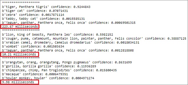
In this example, I have run single inference, but it can speed up more especially on batch execution. (See the following results for reference.)
ResNet-50 Classification with TF-TRT (Azure NCv3, NVIDIA Tesla V100)
| single inference | batch inference | |
|---|---|---|
| General Purpose CPU (Azure DS3 v2) | 694 ms/image | 649 ms/image |
| V100 (Azure NCv3) | 6.73 ms/image | 1.34 ms/image |
| V100 (Azure NCv3) with TensorRT | 3.42 ms/image | 0.47 ms/image |
(Running on : Ubuntu 16.04, CUDA 9.0, cuDNN 7.1.4, Python 3.5.2, TensorFlow 1.8, TensorRT 4.0.1)
Here I have showed you TensorRT inferencing with ONNX conversion to use optimizer.
However, TensorRT Integration (TF-TRT) is already included in native TensorFlow (both v1 and v2) library and you can also use this native method to run inference on TensorRT. (By installing the corresponding version of TensorRT runtime, you can directly convert TensorFlow graph to TensorRT graph with this method.)
See here for this example of TensorFlow-TensorRT Integration (TF-TRT).
For technical details about TensorRT transformations and optimizations, see “NVIDIA Developer Blog : Deploying Deep Neural Networks with NVIDIA TensorRT“.
Note (Added 08/2021) : See here for running TensorRT inference with custom entry script on Azure Machine Learning (AML).
[History]
July 2021 : Updated for the latest TensorRT 8.0
Aug 2021 : Updated contents to use Tesla T4 (from K80)
Categories: Uncategorized

I will really appreciate the writer’s choice for choosing this excellent article appropriate to my matter.Here is deep description about the article matter which helped me more.
machine learning course training in indore
LikeLike