In case you build learner to detect anomalies, it will often be difficult to collect error (outlier) data. This is why one-class support vector machine (one class SVM) matters.
In this post, I show you a brief introduction to one-class support vector machines (one class SVM) in Python code.

In this post, I’ll use OneClassSVM class in scikit-learn, which is used for the unbalanced binary classification. This is the unsupervised learner, i.e, it doesn’t need to know the possible anomalies (outliers) in the training. (The only true (inlier) data is used in the training.)

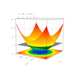
Note : For mathematics behind SVMs, see my post “Mathematical Introduction to SVM and Kernel Methods” (June 2020).

Introduction to OneClassSVM

Now I show you a brief example of this unsupervised learner.

In this example, I have created 500 true data points for training.
As I have said before, this doesn’t include any outlier data.

import numpy as npimport pandas as pdtrain_count = 500train_mem = np.random.normal(size=train_count)width_mem = max(train_mem) - min(train_mem)limit_mem = min(train_mem)train_dsk = np.random.normal(size=train_count)width_dsk = max(train_dsk) - min(train_dsk)limit_dsk = min(train_dsk)traindata = pd.DataFrame({  "AvailableMemory": np.round(200 * (train_mem - limit_mem)/width_mem, 2),  "DiskIO":  np.round(100 * (train_dsk - limit_dsk)/width_dsk, 2),})

The following shows how data (true data) is mapped in space.

import matplotlib.pyplot as pltplt.scatter(traindata["AvailableMemory"], traindata["DiskIO"])plt.xlabel("AvailableMemory")plt.ylabel("DiskIO")plt.show()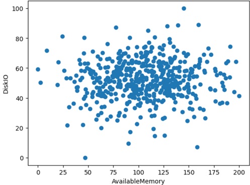

Now I train the model (OneClassSVM) with this training data (500 data points) as follows.

from sklearn import svmmodel = svm.OneClassSVM(kernel="rbf", nu=0.1, gamma="scale")model.fit(traindata.to_numpy())

Note : See here how parameter nu () performs.

Next I generate 10 other data points for test.
This data includes 2 outlier points as follows.

# create test data (10 points)test_count = 10test_mem = np.random.normal(size=test_count)test_dsk = np.random.normal(size=test_count)testdata = pd.DataFrame({  "AvailableMemory": np.round(200 * (test_mem - limit_mem)/width_mem, 2),  "DiskIO":  np.round(100 * (test_dsk - limit_dsk)/width_dsk, 2),})# set outlier data (2 points)testdata.loc[2, "AvailableMemory"] = 100testdata.loc[2, "DiskIO"] = 150testdata.loc[6, "AvailableMemory"] = 0testdata.loc[6, "DiskIO"] = 120

Now I show you how data is mapped.
The green points (total 500 points) are for training and red points (total 10 points) are for test.

import matplotlib.pyplot as pltplt.scatter(traindata["AvailableMemory"], traindata["DiskIO"], c="green")plt.scatter(testdata["AvailableMemory"], testdata["DiskIO"], c="red")plt.xlabel("AvailableMemory")plt.ylabel("DiskIO")plt.show()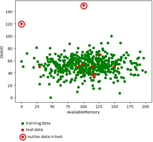

Let’s run prediction on this test data (10 points).
As you can see the result as follows, testdata[2,:] and testdata[6,:] are estimated to be outliers.

pred = model.predict(testdata.to_numpy())print(pred)

array([ 1,  1, -1,  1,  1,  1, -1,  1,  1,  1])

This result (1 or -1) is determined by scores internally, which is based on the distance in hypersphere. (See here for margin maximization in high-dimensional space.)
If you need it, you can also see raw scores as follows.

raw = model.score_samples(testdata.to_numpy())print(raw)

array([15.73642356, 15.96562868,  2.34744343, 14.82687568, 15.57808738,   15.49068674,  3.26862484, 16.00755819, 16.08783021, 16.4708345 ])

Note : The decision (1 or -1) is determined by decision_function() method (in which, positive for an inlier and negative for an outlier), and it can be controlled by dual_coef_ and intercept_ in OneClassSVM class properties.
See here for source code.

The data points are normalized by setting gamma="scale" in OneClassSVM, but the score and the threshold will depend on the problems (e.g, how data is distributed, how far is outliers in high-dimensional spaces, etc), and you should take care when you manually determine whether it’s outlier or not.

Practice (Example) for Real Case

Now let’s see the real scenario.

Here I use the “Breast Cancer Wisconsin Data Set” (download from here), which has 569 samples for patients of breast cancer and candidates.
This data has patient id, diagnostic result of disease (M = malignant, B = benign), and a lot of other attributes computed from a digitized image of a breast mass (such as, radius, texture, perimeter, etc). This example (vector) consists of a lot of dimensions.

8510426, B, 13.54, 14.36, 87.46, ...8510653, B, 13.08, 15.71, 85.63, ...8510824, B, 9.504, 12.44, 60.34, ......

Note : The format of this dataset is well-formed for analysis purpose, but you must run a variety of preprocessing tasks (such as, appropriate attribute’s selection, vectorization, data cleaning, eliminating dependencies, …) in most cases before training.
In this example, we don’t need any extra preprocessing tasks.

Here I train and predict with the following steps.

1. Split the original data into the training purpose (max 450 samples) and test purpose (others).
2. Train and create model by OneClassSVM with training data.
   In training, we remove outlier data (which diagnostic result is ‘M’) and we use attributes except for patient id and diagnostic result (‘M’ or ‘B’).
3. Predict test data by the generated model with test data, and evaluate the results by comparing between true result and predicted result.

This Python code is here.
As you can see the result (ROC curve) as follows, it seems to fairly match the diagnosis results.

import csvimport pandas as pdfrom sklearn import svmfrom sklearn.metrics import roc_curveimport matplotlib.pyplot as plt# Load dataheader=[  "patientid",  "outcome",  "radius_mean",  "texture_mean",  "perimeter_mean",  "area_mean",  "smoothness_mean",  "compactness_mean",  "concavity_mean",  "concavepoints_mean",  "symmetry_mean",  "fractaldimension_mean",  "radius_error",  "texture_error",  "perimeter_error",  "area_error",  "smoothness_error",  "compactness_error",  "concavity_error",  "concavepoints_error",  "symmetry_error",  "fractaldimension_error",  "radius_worst",  "texture_worst",  "perimeter_worst",  "area_worst",  "smoothness_worst",  "compactness_worst",  "concavity_worst",  "concavepoints_worst",  "symmetry_worst",  "fractaldimension_worst"]list_data = []with open("wdbc.data", "r") as f:  reader = csv.reader(f, delimiter=",")  for row in reader:row_dict = {key: value for key, value in zip(header, row)}list_data.append(row_dict)all_data = pd.DataFrame(list_data)# Split datatraindata = all_data.iloc[:450,:]traindata = traindata[traindata["outcome"] == "B"]traindata = traindata.drop(columns=["patientid", "outcome"])testdata = all_data.iloc[450:,:]testdata = testdata.drop(columns=["patientid"])# Train by OC-SVM with true datamodel = svm.OneClassSVM(kernel="rbf", nu=0.1, gamma="scale")model.fit(traindata.to_numpy())# Predict test data with the trained modelresult = model.predict(testdata.drop(columns=["outcome"]).to_numpy())# Evaluate result by visualizing with ROC curvetestdata["true_outcome"] = (testdata["outcome"] == "M")testdata["pred_result"] = resulttestdata["pred_outcome"] = (testdata["pred_result"] == -1)fpr, tpr, thresholds = roc_curve(  testdata["true_outcome"].to_numpy(),  testdata["pred_outcome"].to_numpy())plt.plot(fpr, tpr)plt.xlabel("False Positive Rate")plt.ylabel("True Positive Rate")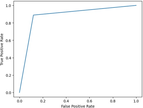

In this post, I have briefly introduced how one class SVM can be used and works well in a lot of anomaly scenarios.

However, you should remember that this learner is “not always” the best choice, but it also has drawbacks.
As you can see here, the model complexity grows when the number of data increases in this algorithm. For this reason, SVM classifier is not then good choice for vast amount of data to train.

Breaking Changes : I have updated this post not to use MicrosoftML (but to use scikit-learn), because Microsoft Machine Learning Server is no longer supported and retired.