
In practical LLM’s training (including fine-tuning), it won’t fit to GPU memories, and it will stuck into the famous “CUDA out of memory”.
The mixture of optimizations – such as, model parallelisms, quantization, algorithm’s optimizations, or compressions – are then usually applied, and the scaling (parallelism) is especially an integral part of LLM training.
The newest NVIDIA’s H100 VM’s series (also A100 VM’s series) has 8 GPUs per a single virtual machine, but a lot more resources are often required for actual LLM’s training (or fine-tuning).
For this reason, the training across multiple nodes is then required in most cases.
For example, OpenAI’s GPT-3 model (which has 175 billion parameters) are estimated to need thousand of GPUs for training 300B tokens within a month by basic technologies (without any optimizations).
Meta’s OPT-175B model has actually used 5,400 GPUs for training in Microsoft Azure.
NVIDIA’s Megatron-LM based 530B model (strictly, Megatron-Turing NLG, shortly MT-NLG) – which is a GPT-3-based model, but fully tuned for GPU devices – is trained on 4,480 GPUs in Azure.
Microsoft Azure is a proven platform, on which these models’ training (including GPT-4 training) are scaled out to thousands of GPUs across multiple nodes. (See “What runs ChatGPT“.)
In this post, I’ll break down the techniques for scaling large models in Microsoft Azure in a step-by-step manner.
Note : Microsoft Azure is the only platform for providing high-speed InfiniBand networking among 3 public clouds.
The benchmark (MLPerf 3.1 Training result) demonstrates the completion of GPT-3 training (with C4 dataset) in four minutes on 10,752 NVIDIA H100 GPUs connected by the NVIDIA Quantum-2 InfiniBand, which is just a 2 percent increase compared to the NVIDIA bare-metal submission, and more than 10x faster than the result of newest TPU v5e. (See here.)
In the supercomputer used in OpenAI ChatGPT training, AMD CPUs are also connected by InfiniBand inter-connection.
Provisioning Infrastructure
Create and configure InfiniBand-enabled VMs
To make the workloads parallel in many GPUs, the GPU-to-GPU communication is a very important factor.
On a single node, multiple GPUs are connected each other with high-speed NVLink technologies, but to make fast inter-node communications, here we configure high-bandwidth Quantum-2 InfiniBand networking for archiving linear scaling.
In Azure, certain VM (virtual machine) series – such as, NC, ND, and H-series – have RDMA-capable VMs with SR-IOV and InfiniBand support. Typically, VM SKU with the letter “r” in its name (such as, “Standard_NC24rs_v3”) contains InfiniBand hardware. (However I note that older SKU such like “Standard_NC24r” doesn’t support SR-IOV hardware for InfiniBand.)
To enable RDMA network, deploy VMs in the same availability set or scale set. (When you use Virtual machine scale sets, configure a scale set in a single placement group.)
For installing and setting-up the InfiniBand driver on Azure, see “How to Setup InfiniBand on Azure” (NVIDIA document).
Note : NVIDIA Quantum-2 InfiniBand can also be used in on-premise in-house or bare-metal resources. (Not depending on cloud-specific technologies.)
Note : Using Ubuntu-HPC VM images (Microsoft) or CentOS-HPC VM images (OpenLogic) with InfiniBand-capable SKUs in Azure Marketplace, these components (such as, GPU driver, InfiniBand drivers, CUDA, NCCL and MPI libraries) are all pre-installed and configured.
Also, in Azure Machine Learning, the compute cluster with InfiniBand-capable SKUs has the pre-configured drivers (including Mellanox OFED driver) to enable InfiniBand. You can save time to prepare environments using pre-configured images in Azure Machine Learning.
Install NCCL and other libraries
NCCL (NVIDIA Collective Communication Library) is a primitive library for both inter-GPUs and inter-nodes communications, which supports a variety of inter-connection technologies including PCIe, NVLINK, and InfiniBand.
A lot of libraries (such as, DeepSpeed) reply on the NCCL backend (not MPI) for the fast GPU communications both within and across nodes.
Installing NCCL is very simple. (See below.)
# Install NCCLwget https://developer.download.nvidia.com/compute/cuda/repos/ubuntu2004/x86_64/cuda-keyring_1.0-1_all.debsudo dpkg -i cuda-keyring_1.0-1_all.debsudo apt-get updateNote : Here I suppose Ubuntu 20.04 and CUDA 12.2. Please change the download packages depending on your environment.
You can check whether NCCL is enabled in PyTorch as follows.
python3 -c "import torch;print(torch.cuda.nccl.version())"Note : Instead of NCCL, you can also use MSCCL (Microsoft Collective Communication Library) to run DeepSpeed. MSCCL abstracts for both NVIDIA GPU stack and AMD GPU stack.
Depending on the library you want to use in workload, please install and set-up other libraries and packages.
For instance, you might setup DeepSpeed library for implementing multi-node’s parallelism.
Cluster management and job scheduling
Job management and scheduling is an integral part for running large and practical jobs.
You can use the following managed services in Microsoft Azure to manage jobs.
| Azure Batch | This service is appropriate to manage primitive cluster scaling and job scheduling for running Batch jobs. |
| Azure CycleCloud | This service is appropriate to bring well-known HPC schedulers (such like, Slurm, OpenPBS, LSF, etc) into Azure cloud. (i.e, Batch services + Scheduler as a Service) Without setting-up login hosts, license servers, and authentications individually, you can use existing skills of familiar schedulers in cloud. |
| Azure Machine Learning | This service is appropriate to operationalize workloads in overall machine learning (ML) lifecycle – such as, scripting training job flows, orchestrating jobs with triggers, and deploying models. This also includes ML specific value-added features – such as, model catalog, evaluating, or monitoring LLMs, etc. Unlike Azure CycleCloud, you should use Azure ML specific commands (CLI) or SDKs. (See here.) |
When you choose InfiniBand-enabled VM in CycleCloud or Azure Machine Learning, InfiniBand settings (such as, installing required software, etc) automatically configured and you can soon start training.
Here I don’t go details about settings for these services, but please refer each document in Azure.
Note : For running machines on Azure Machine Learning, you should need quota for machine learning VMs, which is not for ordinary VMs.
Implement Model Parallelism
In large language models (LLMs), the model cannot be fitted to a single device, including its memory. The model is then usually partitioned into multiple devices, so called “model parallelism”.
In this section, I’ll briefly show you how each strategy of parallelism performs, and also show you the example of implementation for each techniques.
Note : The training data (not model) can also be parallelized across multiple processes (the gradients are then synchronized), and it’s called data parallelism (DP).
The motivation of data parallelism is to speed up training. (On contrary, the motivation for model parallelism is to fit model to the memory.) But, in most cases, model parallelism is also performed with data parallelism together.
Of course, data parallelism itself can also be used alone. In this post, I don’t focus on data parallelism, but see Distributed Data Parallel (DDP) for the implementation in PyTorch.
1. Pipeline Parallel (PP)
For instance, to run model training on 8 devices in a single node, you can simply put layers on multiple devices as following code in PyTorch. (In the following example, I assign 8 GPU devices, cuda:0, cuda:1, … and cuda:7 to each layer.)
Pipeline parallelism (PP) is based on this kind of layer-level (block-level) partitioning.
import torch.nn as nnclass MyAttention(nn.Module): def __init__(self, features_dim):... def forward(self, x):...class TestModel(nn.Module): def __init__(self):super(TestModel, self).__init__()self.emb = nn.Embedding( num_embeddings=10000, embedding_dim=128,).to("cuda:0")self.attn_layers = nn.ModuleList([ MyAttention(features_dim=128).to(f"cuda:{i+1}") for i in range(6)])self.head = nn.Linear(128, 10000).to("cuda:7") def forward(self, x):x = self.emb(x.to("cuda:0"))for i, attn in enumerate(self.attn_layers): x = attn(x.to(f"cuda:{i+1}"))return self.head(x.to("cuda:7"))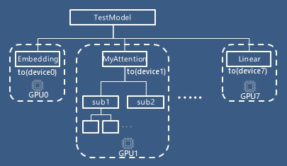
However, when it’s performed by regular sequential fashion, only one device will be active at a time and GPU utilization will suffer.
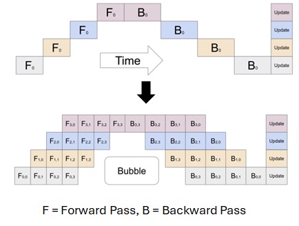
To prevent this kind of inefficient utilization, each computations in partitions should then be scheduled to perform by parallel execution. In pipeline parallel, it splits training batch into multiple micros-batches, and these can be executed in pipelined stages. (See below.)
From : GPipe: Efficient Training of Giant Neural Networks using Pipeline Parallelism
Note : Pipeline scheduling is also complemented with data parallelism to further scaling.
The optimizer steps are then synchronized across devices.
Pipeline bubble (see above) is the idle time at the start and end of every batch, which should be as small as possible.
In Megatron-LM, the pipeline is executed by the interleaved scheduling as follows to make the size of the pipeline bubble smaller. (See below.)

From : Efficient Large-Scale Language Model Training on GPU Clusters Using Megatron-LM
Pipeline parallelism requires code integration with the definition – such as, partition’s boundaries, topologies, and resource assignment’s strategy.
For instance, the PipelineModule class in DeepSpeed library (see here) simplifies the implementation of pipeline parallelism.
The following example shows that there are 4 x 1 = 4 GPUs available in total and the model is partitioned into 8 layers.
By specifying partition_method="parameters", GPU resources are assigned into layers depending on the number of parameters in layer. For instance, if some layer has large number of parameters, large resources will then be assigned.
from deepspeed.pipe import PipelineModule, LayerSpecfrom deepspeed.runtime.pipe import ProcessTopology...layer_specs = []layer_specs.append(LayerSpec(nn.Embedding, num_embeddings=10000, embedding_dim=128))for i in range(6): layer_specs.append(LayerSpec(MyAttention, features_dim=128))layer_specs.append(LayerSpec(nn.Linear, 128, 10000))topology_specs = ProcessTopology(axes=["x", "y"], dims=[4, 1])model = PipelineModule( layers = layer_specs, loss_fn = nn.CrossEntropyLoss(), topology = topology_specs, partition_method = "parameters", activation_checkpoint_interval = 0)Note : In some language models (such as, BLOOM, GPT 2 with LM head, etc), the weights of embedding are shared with the linear layer of the language modeling head. In such case, you can use
TiedLayerSpec(instead ofLayerSpec), in which you can specifykeyfor the identification of weight’s sharing.Note : If you don’t need to store the type information and parameters for each stage, you can also bring your model without using
LayerSpecclass (without modification) and simply usePipelineModuleclass with your model implementation. (Each step andtorch.nn.Sequentialin model is automatically flatten into each stages.)Note : With Varuna (also developed by Microsoft Research), pipeline parallelism can also be transparently implemented by defining partition boundaries (by Varuna’s
CutPointobject).
2. Tensor Parallel (TP)
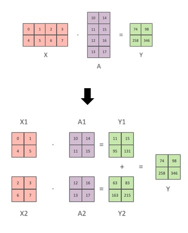
Tensor parallel (shortly TP, or tensor slicing) is the parallelism technique by the tensor-level partitioning.
For instance, when you compute the following matrix multiplication 


As a result, each device will only need the half of tensors.
The layers – such as, multi-layer perceptron (MLP) block – are considered to be matrix multiplication, and these layers can also be partitioned into parts.
From : Hugging Face “Model Parallelism“
Note : This paradigm is also complemented with data parallelism to further scaling. (See above note for data parallelism.)
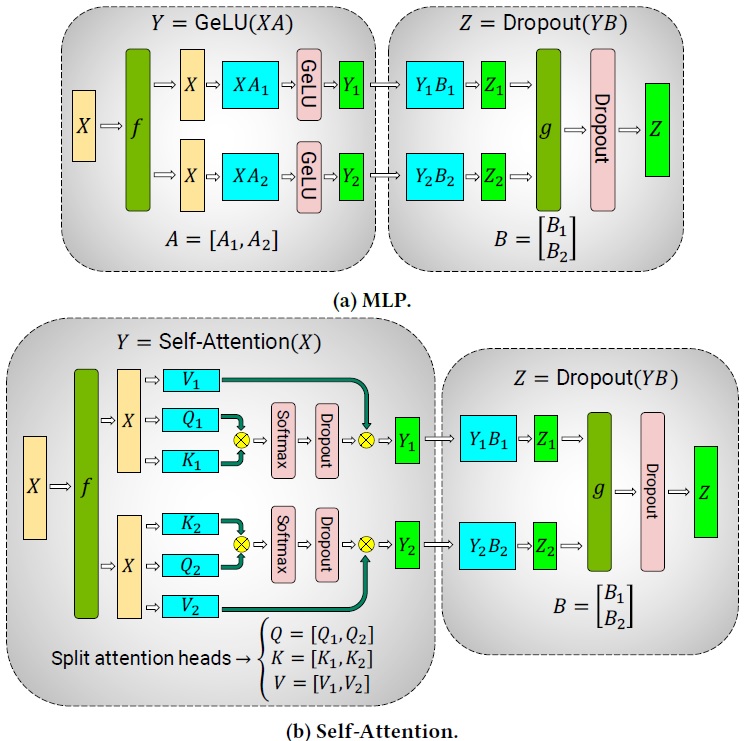
One of the famous TP implementation is Megatron-LM. (In this work, the combination of both pipeline parallelism and tensor parallelism is applied in the model implementation.)
In Megatron-LM, multi-layer perceptron (MLP) block with GeLU activation (which follows a self-attention block) in transformer is parallelized by tensor slicing. Furthermore, the multi-head attention operation is also parallelized by partitioning key, query, and value matrices in transformer. (i.e, The matrix multiplication corresponding to each attention head is done on a single GPU.)
From : Efficient Large-Scale Language Model Training on GPU Clusters Using Megatron-LM
Note : In Megatron-LM, data parallelism is also applied.
To say, Megatron-LM implements the mixture of parallelism – tensor parallelism (TP), pipeline parallelism (PP), and data parallelism (DP). This architecture of mixture is called 3D parallelism.
In general, tensor parallelism requires extensive code integration that may be model architecture specific.
See here for the implementation of tensor parallel (TP) in Megatron-LM.
Note : NVIDIA NeMo framework includes platform called NeMo Megatron, which is inspired by Megatron-LM model. It provides 3 types of model parallelism – tensor parallelism, pipeline parallelism, and sequence parallelism.
You can also use NVIDIA NeMo framework in Azure Machine Learning.Note : See here (Megatron-DeepSpeed) for DeepSpeed version of NVIDIA’s Megatron-LM implementation.
3. Mixture-of-Experts (MoE) – Expert Parallel
Mixture-of-Experts (MoE) is not a parallelism technique, but is a generally used method in machine learning for ensemble combination, in which each expert performs a specific subtask and all experts are then weighted to get the final result.
In this technique, both experts and weighting functions are then trained.
Today sparse MoE is widely used in large neural networks. Let’s see the following popular architecture, called Sparsely-Gated MoE :
- The gating network is used for selecting a few experts.
In the following picture, the gating network is used to select only 2 experts. - Each expert consists of a simple feed-forward network.
- The outputs of experts are then weighted, in which the weights are determined by the previous gating network.
- Multiple MoE layers are stacked. (See the left side in the following picture.)
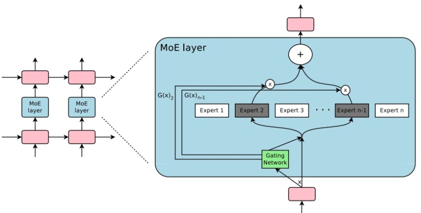
From : “The Sparsely-Gated Mixture-of-Experts Layer”
Note : Many routing algorithms are proposed to maximize model accuracy.
By selecting a few experts (in this example, 2) in each stacking layer, it significantly reduces computations at a time, while it has the same budget as a dense model.
This is why the name implies “sparsity”.
Note : In general, MoE architecture can be dense or sparse.
Note : The sparse MoE architecture is resource-effective compared with fully dense models, but not equivalent to fully dense models of same size in terms of accuracy.
The research result (see here) says that the fully dense model generally outperforms sparse MoE model of same size in terms of model’s accuracy. (It’s an active research area.)
In LLMs, MoE architecture replaces Transformer’s feed-forward layers (Multi-Layer Perceptrons (MLPs) or attention projection) with sparse MoE layers. As you know, Transformer has multi-layered architecture (see here) and these MoE layers are then stacked in natural way.
See GShard or Switch Transformers for the architecture of applying MoE in LLMs.
Note : See this tweet for three types of Mixture of Experts (MoE) – Pre-trained MoE, FrankenMoE, and Upcycled Fine-grained MoE.
The sparse MoE in LLMs reduces GPU hours, and eventually more tokens can be processed in fixed time or compute’s cost constraints. It also gives much faster pre-training and inferencing due to fewer activated parameters.
Each reduced workload can also be parallelized by assigning each experts to different devices. (Expert parallelism)
OpenAI doesn’t publicly mention, but GPT-4 is rumored to be trained on MoE layers.
Mixtral 8x7B is also a famous language model built with a sparse MoE network which has 8 experts.
The sparse MoE is now gathering much attentions in LLMs.
To implement MoE, it also requires extensive code integration that may be model architecture specific.
With DeepSpeed library, you can use deepspeed.moe.layer.MoE to simplify this implementation. (See here for Megatron-DeepSpeed implementation.)
See OpenMoE repository for the implementation of open-sourced MoE LLMs.
4. Zero Redundancy Optimizer (ZeRO)
In the training, the large number of memory holds the optimizer states, gradients, and parameters compared to the inference – in which all sizes are depending on the number of parameters. (Especially, the optimizer states will hold a large part of memory, depending on the precision and the kind of optimizers.)
In ZeRO-powered data parallelism (shortly, ZeRO-DP), model is trained in each node by data parallel fashion, while each device stores only a horizontal slice of these memories – optimizer states, gradients, and parameters.
The model is then granularly divided into partitions in the training.
The following video shows how ZeRO-DP performs.
From : ZeRO & DeepSpeed: New system optimizations enable training models with over 100 billion parameters
Steps
- The training data is divided into each partition. (i.e, Data parallelism)
- Each partition holds only a part of parameters. (Parameters are distributed and partitioned.)
- The forward pass in the training is processed using each divided data, but it needs all parameters to process in each partition. Therefore, the missing parts of parameters are then shared (synced) across partitions in each step.
- In backward pass, the gradients in each step are computed by estimating the loss, and then each partition has the computed gradients for corresponding data. Therefore, the computed gradients for all data is accumulated into each corresponding partitions.
Eventually each partition will then have a part of parameters and corresponding gradients. - Finally, the optimization is processed using parameters and the computed gradients.
In this stage, the optimization can be processed by parallel in each partition. (Because parameters and the corresponding gradients resides in the same partition.) - The updated parameters (new parameters) are stored into the corresponding partition.
The new parameters are then used in the next iteration … (Go to 1 again …)
Note : In DeepSpeed, you can configure either of the following 3 stages (strategies) of partitioning.
- optimizer states partitioning
- optimizer states + gradient partitioning
- optimizer states + gradient + parameter partitioning
One of important aspects of ZeRO optimization is that you don’t need to modify the model implementation, because the model is parallelized in runtime.
For example, here is the source code for fine-tuning with ZeRO-DP, in which I have downloaded pre-trained Meta’s OPT model from Hugging Face. As you can see below, the downloaded OPT model can be used in ZeRO without any modification.
import torchfrom torch.utils.data import DataLoader, DistributedSamplerfrom torch.optim.lr_scheduler import LambdaLRfrom transformers import AutoModelForCausalLM, AutoConfig, AutoTokenizer, DataCollatorForLanguageModelingfrom datasets import load_datasetimport argparseimport mathimport osimport deepspeedfrom deepspeed.ops.adam import FusedAdamos.environ["TOKENIZERS_PARALLELISM"] = "false"# Deepspeed launcher passes "local_rank"parser = argparse.ArgumentParser(description="My training script")parser.add_argument( "--local_rank", type=int, default=-1, help="local rank passed from distributed launcher")parser = deepspeed.add_config_arguments(parser)args = parser.parse_args()model_name = "facebook/opt-6.7b"dataset_name = "Dahoas/rm-static"num_epochs = 2train_micro_batch_size_per_gpu = 16gradient_accumulation_steps = 8ds_config = { "train_micro_batch_size_per_gpu": train_micro_batch_size_per_gpu, "gradient_accumulation_steps": gradient_accumulation_steps, "steps_per_print": 10, "zero_optimization": {"stage": 3,"cpu_offload": False, }}# Get devicetorch.cuda.set_device(args.local_rank)device = torch.device("cuda", args.local_rank)# Initialize backend in DeepSpeedtorch.distributed.init_process_group(backend="nccl")deepspeed.init_distributed()# Load modelmodel_config = AutoConfig.from_pretrained(model_name)model = AutoModelForCausalLM.from_pretrained( model_name, config=model_config,)# Get tokenizertokenizer = AutoTokenizer.from_pretrained( model_name, fast_tokenizer=True)tokenizer.pad_token = tokenizer.eos_tokentokenizer.padding_side = "right"# Here I simply use prompt/response dataset in English# (Use other dataset for other languages)dataset = load_dataset(dataset_name)# Filter dataset not to exceed the length 512# (model_config.max_position_embeddings is 2048 in OPT)max_seq_len = 512dataset = dataset.filter(lambda d: len(d["prompt"] + d["chosen"]) < model_config.max_position_embeddings)# Convert datasetdef _align_dataset(data): all_tokens = tokenizer([data["prompt"][i]+data["chosen"][i] for i in range(len(data["prompt"]))],max_length=max_seq_len,padding="max_length",truncation=True,return_tensors="pt") return {"input_ids": all_tokens["input_ids"],"attention_mask": all_tokens["attention_mask"],"labels": all_tokens["input_ids"], }dataset = dataset.map( _align_dataset, remove_columns=["prompt", "response", "chosen", "rejected"], batched=True, batch_size=128)# Here we use only train datasetdataset = dataset["train"]# Set up optimizer manually# (You can also set up optimizer with DeepSpeed configuration.)optimizer = FusedAdam( params=model.parameters(), # divide into weight_decay and no_weight_decay if needed lr=1e-3, betas=(0.9, 0.95))# Build cosine scheduler manually# (You can also use DeepSpeed built-in scheduler in configuration.)num_update_steps = math.ceil(len(dataset["input_ids"]) / train_micro_batch_size_per_gpu / gradient_accumulation_steps)def _get_cosine_schedule( current_step: int, num_warmup_steps: int = 0, num_training_steps: int = num_epochs * num_update_steps): if current_step < num_warmup_steps:return float(current_step) / float(max(1, num_warmup_steps)) progress = float(current_step - num_warmup_steps) / float(max(1, num_training_steps - num_warmup_steps)) return max(0.0, 0.5 * (1.0 + math.cos(math.pi * progress)))scheduler = LambdaLR(optimizer, lr_lambda=_get_cosine_schedule)# Label is shifted by one element in DataCollatorForLanguageModelingdata_collator = DataCollatorForLanguageModeling(tokenizer=tokenizer, mlm=False)# Initialize components (except for scheduler)model_engine, optimizer, dataloader, _ = deepspeed.initialize( model=model, config=ds_config, optimizer=optimizer, args=args, # lr_scheduler=scheduler, # see below note training_data=dataset, collate_fn=data_collator, dist_init_required=True)# Run train loopfor epoch in range(num_epochs): model_engine.train() for i, batch in enumerate(dataloader):batch = {k:v.to(device) for k, v in batch.items()} # send to GPUwith torch.set_grad_enabled(True): outputs = model_engine(**batch) loss = outputs.loss model_engine.backward(loss) model_engine.step() # Note : Here I manually step scheduler, # but you can also set scheduler in deepspeed.initialize() # when it's supposed to execute at every training step. if model_engine.is_gradient_accumulation_boundary():scheduler.step() print(f"Epoch {epoch+1} {math.ceil((i + 1) / train_micro_batch_size_per_gpu / gradient_accumulation_steps)}/{num_update_steps} - loss: {loss :2.4f}", end="\r") print("")Note : You can also configure ZeRO-Offload or ZeRO-Infinity, which offloads memory data (such as, parameters, etc) into CPUs or NVMe memory.
Seeoffload_optimizerandoffload_paramparameters in DeepSpeed’s document.
DeepSpeed library is also integrated with Hugging Face transformer’s Trainer class. So you can easily configure model parallelism even in Hugging Face’s Trainer as well.
Also, see Fully Sharded Data Parallelism (FSDP) in PyTorch (see here), which is also inspired by ZeRO Stage 3 and shares the optimizer states, gradients and parameters across devices.
In this post, I have only focused on model scaling, but reducing memory (resource’s optimization) is also an important aspect and various techniques are used in practical training or fine-tuning. For instance, the number of GPUs can be reduced approximately to one-fourth by applying LoRA in finetuning for a simple task. (See here for the implementation of LoRA.)
Both scaling and resource’s optimization are usually applied together, and become an integral part of practical large training.
Reference :
What runs ChatGPT ?
https://techcommunity.microsoft.com/t5/microsoft-mechanics-blog/what-runs-chatgpt-inside-microsoft-s-ai-supercomputer-featuring/ba-p/3830281
Categories: Uncategorized

1 reply»