In this post, I’ll briefly summarize how data is processed in Kusto (Data Explorer) engine – which is implemented as Azure Data Explorer (ADX), Synapse Data Explorer (Synapse DX), or Kusto free.

Note : I also hope that this post will give you a hint for which one to choose among 3 different analytical pools in Azure Synapse – Spark pool, Dedicated SQL pool, or Data Explorer (DX) pool.
See below for other platform architectures.

• Synapse Analytics dedicated SQL pool (Data warehouse)
• Cosmos DB

Note : You can also run Kusto on local docker runtime with Kusto Emulator. (Kusto Emulator is a container image exposing a Kusto Query endpoint.)
You can use it for local development.

Concepts – Optimized for ad-hoc query with large data volumes

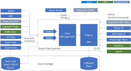
Before I’ll go dive into details, let’s see how you can use Data Explorer.

Data Explorer is optimized for time-series and ad-hoc query analytics – such as, log analytics, IoT, or general telemetry analytics.
Data Explorer assumes historical (time-series) data, and data is well governed and controlled by timestamp value. (By default, it uses ingestion time of arrival for timestamp value.) It can also natively support time-based features, such as, retention setting, windowing, anomaly detection, time-series forecasting, etc.

Like Synapse Analytics SQL pool (data warehouse), Data Explorer can also handle a large volume of data (i.e, limitless data). Same as other big data platforms, data will be processed by scaled manners – such as, hashing, caching, or columnar compressions.
However, Data Explorer has its own standpoint for data analytics.

As I’ve described in my old post, you will define detailed business schema in Synapse Analytics SQL pool (data warehouse), depending on data access patterns. For instance, you might design multiple tables between transactions and dimensions with a lot of relationships, and tune schema by defining the corresponding distribution strategies (REPLICA, HASH, or ROUND-ROBIN) or index strategies. You might also define detailed constraints, such as, string length, not-null constraints, foreign key constraints, etc.

On contrary, Data Explorer also has table and column definitions, but detailed relationships, strategies, and constraints are not set.
Unlike business database, schema won’t be strictly normalized between transactions and dimensions – such as, “Sales” transaction table combined with “City” table by “CityKey”. The table can even hold JSON value without parsing into scalar values. (You can parse the ingested data in Data Explorer, but it’s optional.)
You won’t also explicitly indicate “which table has which index”. (By default, Data Explorer builds indexes for all fields (even when it’s JSON column) in tables.)
Data is then quickly analyzed and visualized in Azure Data Explorer Web UI, Kusto Explorer (Kusto.Explorer), or Synapse Studio.

Data Explorer is optimized for :

• Sliding window to a subset of chronological data
• Read-many
• Insert/append-many
• Delete-rarely (bulk delete only)
• Update almost never

Data Explorer also involves some sort of ETL processing.
Data Explorer can ingest diverse data in both batch ingestions and streaming ingestions.
By default, it can support many ingestion sources (such as, Azure blob, Data Factory, Event Hub, and Event Grid), and you can also collect data from other sources with ADX plugins (such as, Apache Kafka, 3rd party logging tools, etc).

Note : See here for the difference between Azure Data Explorer (ADX) and Synapse Data Explorer pool (Synapse DX).

Architecture Outline

In Data Explorer, data and index are stored in Azure Blob and controlled (managed / queried) by Azure Virtual Machines (engine service and data management service).
Data and index are also cached across nodes on local SSD or even RAM. In most cases, Data Explorer queries data and index available in SSD or RAM.

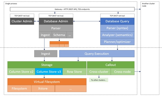
(From “Azure Data Explorer performance update (EngineV3)” in official docs)

Note : VMs in Data Explorer can also access data in a different cluster (so called, cross-cluster query).

Engine service is responsible for running query and some control commands (such as, data ingestions and managements), and it then exposes JSON API endpoints.
As you will find in this post, data is distributed by a lot of shards in Azure Storage containers. Hence, by scaling compute’s layer, data processing can be vastly parallelized across these data blobs.
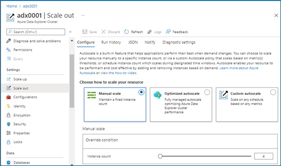
Engine cluster can be scaled manually and automatically (auto-scaling).

As you will find in this post, data is also processed and managed by the background process. Data management (DM) service is responsible for the invocation of these periodic data grooming tasks.

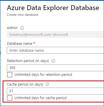
As you saw in the previous section, Data Explorer assumes time-series data, and by default, Data Explorer uses ingestion time (ingested in-order of time of arrival) for this timestamp value.
Based on this timestamp value, data will be controlled in the management – such as, retention, partitioning, and caching. (See here for cache policy setting.)

Note : You can specify custom creationTime for ingestion timestamp.

Data shards (extents) and column store

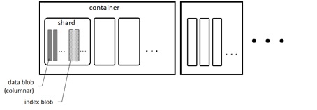
As you saw in the previous section, data is stored in Azure Blob service.
Each data is divided into a number of extents (data shards) and each extent holds column store (columnar compression) of data.
Extents are distributed in multiple containers in Azure Storage, and operations can then be balanced across storage.

The extents are maintained by data management (DM) service periodically in background.
Some large extent might be generated in a single ingestion. However, if the number of rows exceeds some threshold (1,048,576 by default), the extent will be divided into multiple extents.
On the other hand, when you have repeatedly ingested data, the extents will be separated by small chunks after ingestion. However, these extents will eventually be merged.

Note : You can see the max row count setting in .show table [TABLE NAME] details command. (See ShardEngineMaxRowCount property.)

For instance, when you ingest some small data twice in table, you will see the following 2 extents after ingestion.

.show table StormEvents extents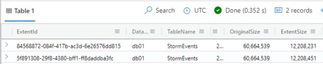

After a while, these extents will be merged into a single extent.

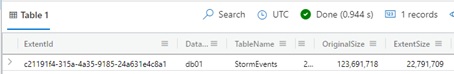
This merge policy (settings) can be seen by running the following command.
(To change merge policy, please run .alter database [DATABASE NAME] policy merge. This command is immediately take effects in database.)

.show database db01 policy merge

"PolicyName": ExtentsMergePolicy,"EntityName": [db01],"Policy": {  "RowCountUpperBoundForMerge": 16000000,  "OriginalSizeMBUpperBoundForMerge": 0,  "MaxExtentsToMerge": 100,  "LoopPeriod": "01:00:00",  "MaxRangeInHours": 24,  "AllowRebuild": true,  "AllowMerge": true,  "Lookback": {"Kind": "Default","CustomPeriod": null  }},"ChildEntities": [  "StormEvents"],

Note : In Data Explorer, there exist 2 types of merging – one (called Merge) is only for index merging, and the other (called Rebuild) includes data artifacts’ merging.
By default, Rebuild is enabled in DX.

In streaming-ingestion enabled tables, data is first stored in row store (not column-compressed) at ingestion. When data exceeds some threshold in row store, the data is automatically moved into column store.
When you run query for this table (including data in both row store and column store), the query will be processed for both stores and the result is combined. (This is transparent for users.)

Note : Remind CCI in Synapse Analytics dedicated pool (data warehouse). The inserted data is temporarily stored in rowstore table (called delta store), when you add row without loader. When data exceeds some threshold (around 1 million rows), it will then be compressed and put into column store.

Query processing

When you submit some query written by Kusto Query Language (KQL), the query analyzer parses into Abstract Syntax Tree (AST) and builds an initial Relational Operators’ Tree (RelOp tree). It then finally builds a query plan as follows.

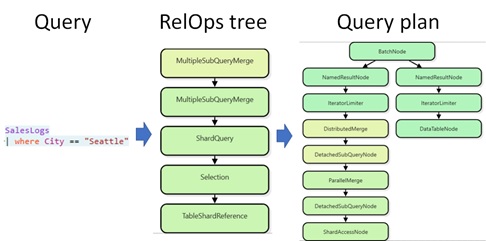
Note : You can see these plans in Kusto Explorer (Kusto.Explorer). (Select “Tools” – “Query Analyzer” command.)

The generated plan is eventually translated into the distributed query plan, which is a shard-level access tree. (See below.)

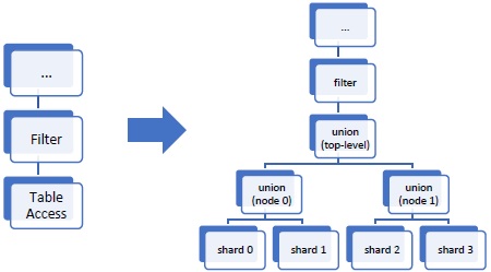
(From “Data Explorer whitepaper“)

Note : To optimize concurrency, please configure the request rate limit policy. (See here.)
By default, maximum concurrency (MaxConcurrentRequests) is limited to {cores-per-node} x 10 in a single workload group.

In join or summarize (group-by key) query, the data movement will also be needed.
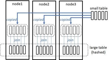
In join operations, the query optimizer estimates the size (the number of rows) and cardinality (the number of distinct keys) in both join sides, and will then decide one of the following strategies.

• Broadcast join strategy :
  If one of join sides is significantly smaller than the other, this small table will be distributed (broadcasted) to all nodes, and it will then perform hash joins on each node in parallel.

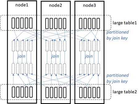
• Shuffled join strategy :
  If both join sides are large, it will apply same partitioning scheme for both sides (data is then shuffled) and perform hash joins within each partition.

• Other :
  Both join sides are not so large (similar size and cardinality), it will bring both sides to the same node and perform non-distributed joins.

Note : The shuffle strategy is also used in summarize query, and the aggregation operation is then distributed into all nodes. (Broadcast strategy is not applied in summarize query.)
Data Explorer has its own data shuffling mechanism to parallelize join/summarize operations. See whitepaper for data movement strategies and SelectPartition operator.

Note : You can also specify a hint to force strategies in query. (Below example forces broadcast strategy.)

CustomerActivityLogs| join hint.strategy = broadcast (SalesLogs) on CustomerKey| top 20 by SalesPrice desc

Partitioning

By default (when partitioning policy is not assigned), extents are partitioned by ingest-time based partitioning.
Specifying your own partitioning policy in table is not mandatory (it’s optional), however, if you need, you can leverage this feature by custom partitioning policy.

First let me introduce hash partitioning.
Now I assume that we specify the following partitioning policy in SalesLogs table.

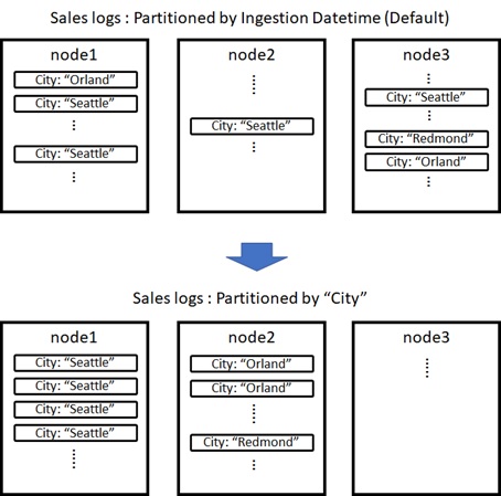
.alter table SalesLogs policy partitioning ```{  "PartitionKeys": [{  "ColumnName": "City",  "Kind":"Hash",  "Properties": {  "Function": "XxHash64",  "MaxPartitionCount":128,  "Seed": 1,  "PartitionAssignmentMode":"Default"  }}  ]}```

By setting this custom policy, the extents in this table will be re-partitioned by the hash of City. This will be run in the background process after data ingestion.
In this example, by setting “Default” in PartitionAssignmentMode, all homogeneous extents (i.e, the extent which has the same hash value) will be assigned to the same node. (See below.)

Note : Please wait till data is partitioned by the background process. Once data is partitioned, you can see the distributed extents by running the previous .show table [TABLE NAME] extents command.
When you change the partitioning policy for existing table, please clear data and re-ingest all data under new partitioning policy.

The benefits of partitioning is for query optimizations.
In query execution, it will speed up by filtering by the partition value. For instance, when you run query filtering by City in this table, the engine service can directly access the target partitions without scanning data.
Another example is for join/summarize (aggregations) operations. When you run join/summarize operations by City column, the data movement across nodes won’t be needed. (Because the data which has the same hash exists in the same node.)
When you or your app always filter data with some specific column (such as, “tenant id” in SaaS application), please consider to apply custom partitioning policy to speed up.

The partition policy can be assigned for datetime and string columns.
For datetime column, you can assign the uniform range partitions instead of hash partitions, in which each extent belongs to the partition with the limited time range. (The default partitioning policy uses this type of partitioning for ingestion time value.)

Note : When OverrideCreationTime property is set to true in uniform range partitioning, retention and caching policies are also aligned with this datetime value.

You should take care to assign custom partitioning policy, because it will affect entire performance in query for this table.
See here for details about partitioning policy.

Other topics for data sharing and distributions

Finally, I’ll describe a few topics about query optimizations. These are optional, but will also improve query concurrency in some cases.

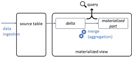
– Materialized View

Like Synapse Analytics SQL pool (see here), you can also use a materialized view in Data Explorer, in which the aggregations are pre-computed, stored, and maintained in database.
Querying a materialized view is more performant than the query for source table, in which the aggregation will be performed each query.

The result of materialized view is always up-to-date.
When the new data is ingested into the source table, the data is kept as “data that haven’t yet been processed”. Querying against a materialized view combines “data that have already been processed” (called “materialized part”) and “data that haven’t yet been processed” (called “delta”).
After a while, the background process will process “delta” and merge into “materialized part”.

– Query results cache

When you enable results cache in the query as follows or as a client request property, the result is cached in its own private storage and the subsequent executions for the same query then get results directly from this cache.
By the following setting, the result cache is used within 5 minutes, and the query is processed (and the cache is saved again) over 5 minutes.

set query_results_cache_max_age = time(5m);SalesLogs| where SalesDate > ago(365d)| summarize arg_max(SalesPrice, *) by Id

Note : The query result is cached. Do not confuse with above cache mechanism for data itself.

Note : If the cached data in private storage exceeds capacity, it’s automatically evicted by LRU (least recently used) policy.

When some query is repeatedly submitted and you don’t need real-time results (or staleness is allowed), you can improve performance by enabling result cache.
Such as materialized view, especially you can save resources for query processing, when the query workload consumes high-cost.

I note that the cache in storage resides in each node, and not shared across nodes in the cluster.

Note : When you have enabled row level security, the results of query cannot be cached. See here for compatible queries in query results cache.

– Leader-Follower Pattern

In Data Explorer, you can also use leader-follower pattern for distributing query workloads across multiple clusters.
When follower database in a different cluster is attached to the original database called “leader” database, the follower database will synchronize changes in leader database. With read-only follower database, you can view data of the leader database in a different cluster. (The followers must be in the same region with leader.)

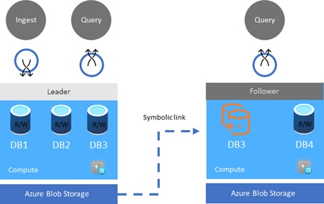
You can use this pattern for the scale-out purposes in large system.
You can also specify different SKUs and caching policies in follower clusters. You can distribute the read query workloads into multiple clusters, especially when heavy ingestion’s workload occurs in leader database.

Reference :

Azure Data Explorer technical white paper
https://azure.microsoft.com/en-us/resources/azure-data-explorer/