Important Note : The retirement of Project Bonsai has been announced. (See here for downloading your data from Bonsai.)

Project Bonsai is a reinforcement learning framework for machine teaching in Microsoft Azure.

In generic reinforcement learning (RL), data scientists will combine tools and utilities (such like, Gym, RLlib, Ray, etc) which can be easily customized with familiar Python code and ML/AI frameworks, such as, TensorFlow or PyTorch.
But, in engineering tasks with industrial machine teaching for autonomous systems or intelligent controls, data scientists will not always explore and tune attributes for AI. In successful practices, the professionals for operations or engineering (non-AI specialists) will tune attributes for some specific control systems (simulations) to train in machine teaching, and data scientists will assist in cases where the problem requires advanced solutions.

Project Bonsai gives us a toolchain for this machine teaching workloads and lifecycle.

In this post, I’ll show you Project Bonsai – how it works and how it simplifies reinforcement learning in machine teaching.

Reinforcement Learning and CartPole example

If you are new to reinforcement learning (RL), please read this section beforehand.

The notable advantage in RL is that it’s the algorithm to find optimal trajectories for actions. (In this post I don’t go so far about RL algorithms, but please see here for details.)
In generic machine learning (so called, supervised learning), the learner will be trained using data, which is prepared before training. However, in practical reinforcement learning (RL), the learner (i.e, agent) will collect data and decide which action is optimal over the course of training. The trajectory for the goal will also be optimized over the course of training and the collected data will then also be refined over the course of training.

In most RL approaches, data scientists don’t need to collect data in advance, but they should design action, state, and reward in order to act this proactive self-training.
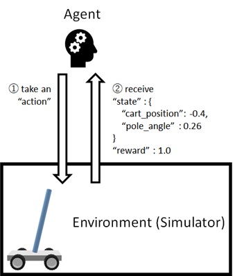
When some action is taken by agent, the corresponding state and reward will be returned from environment. (See below.)

Note : I note that there exists an approach to use pre-collected (prepared) dataset in RL. Bonsai also supports training AI with datasets (Machine Teaching datasets) that you already have.
Such like supervised learning, data scientists should also determine algorithms and hyper-parameters even in RL.

The agent will then learn which action in which state will maximize cumulative rewards. (In most RL algorithms, this learning will not be triggered in each action, but triggered in some amount of collected data, called “batch”.)
By executing this iterations, the agent will finally work as expected, if the design is successful. (See here for Minecraft example.)

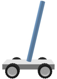
CartPole environment is a widely used and primitive example for RL entry users.
CartPole has a standing pole on a cart and the agent asks AI to move a cart while keeping an upright pole balanced in the center of the cart.

In our Bonsai example, we use the custom Cartpole implementation in Python. (See here for source code.)

sim = cartpole.CartPole()# Reset episodesim.reset(...)# Post actionsim.step(...)# Access states = sim.state

In this custom CartPole, it has an action, which value is a scalar number between -1.0 and 1.0 (inclusive) and it means a force magnitude (i.e, a unit is 1 Newton). On the other hand, the state is a composite of numbers (i.e, structure) – with cart position (meter), pole angle (radian), cart velocity (meter/sec), and pole angular velocity (radian/sec), etc.

In CartPole problem, the state of falling (i.e, exceeding some range in pole angle) or moving out (i.e, exceeding some range in cart position) will be considered as failure and the trial will be terminated.
On contrary, when the agent keeps a pole balanced in 200 trials, this situation will be considered as success and also iterations will be ended at 200 iterations.
This 1 story (maximum 200 iterations) is called an episode in reinforcement learning.
In CartPole problem, the returned reward will always be 1.0. Thus, when it succeeds, the agent will get total 200.0 rewards (maximum rewards) in each episode.

To summarize the motion of CartPole agent :

1. First the agent will receive initial state – cart position, pole angle, cart velocity, etc.
2. By seeing the current state, the agent will then select and perform the next action.
3. The environment returns the result’s state (cart position, pole angle, …) and reward (always 1.0) to the agent.
4. By checking the returned state, the agent will then select and perform the next action again.
   But, if it’s end state, the episode is terminated and go into the next episode. (Go to 1.)
5. To be repeated …

By reinforcement learning algorithms, this agent can learn to maximize cumulative rewards (i.e, to take 200.0 rewards) in a episode.

Note : See here (my GitHub repo) for CartPole examples with a variety of RL algorithms in Python.
In this Gym-integrated CartPole-v0 environment, the value of action is discrete – 0 (push left) or 1 (push right). Therefore it can be handled in basic reinforcement learning algorithms, such as primitive Q-learning (not DDPG), for entry users.
Today’s popular algorithms – such as, PPO, SAC, etc – can handle continuous actions and observations. Bonsai also uses these modern algorithms.

Before we start

In order to see how Bonsai works with simulators and connectors, I first provision a local simulator which runs custom code in Python, and connect to cloud Bonsai workspace.
Before staring, please set up Bonsai workspace (cloud) and local environment as follows.

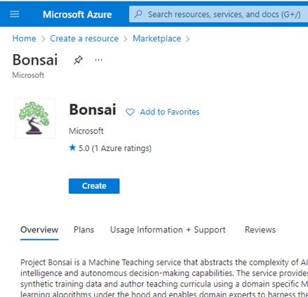
First, create a Bonsai resource (i.e, Bonsai workspace) in Azure Portal.

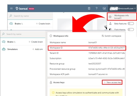
Open Bonsai workspace UI (https://preview.bons.ai/), and click your e-mail on the top-right corner, and select “Workspace info”. (See below.)
In the screen, please create access key, and copy workspace id and access key. (These values will be used in the following steps.)

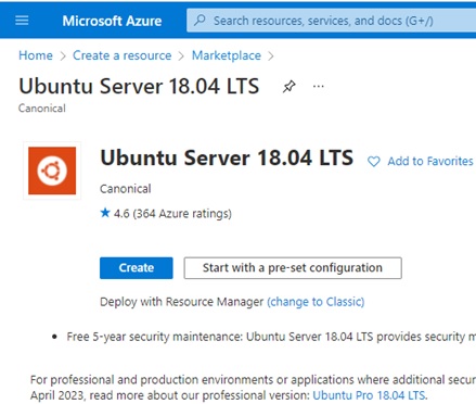
To run a local simulator, please create a Ubuntu VM (virtual machine) resource in Microsoft Azure. (Here I used Ubuntu 18.04 LTS.)

Install Bonsai CLI on Ubuntu VM as follows.

# Check whether Python 3 is installedpython3 -V# Set up pip3sudo apt-get updatesudo apt-get install -y python3-pipsudo -H pip3 install --upgrade pip# Install Bonsai CLIpip3 install bonsai-cli

Logout / login again, and run the following command. (Replace a placehold {BONSAI-WORKSPACE-ID} with your Bonsai workspace id.)
This command will make your local environment (on Ubuntu) connected to your cloud workspace. (The configuration is written on ~/.bonsaiconfig file.)

# Run once in your working environmentbonsai configure -w {BONSAI-WORKSPACE-ID}

Also, install Bonsai Platform API for Python as follows, because we will run a simulator program with Bonsai API later.

pip3 install microsoft-bonsai-api

Run Local Simulator (Unmanaged Simulator)

Next I’ll run my local simulator (custom code) on Ubuntu VM, and connect to Bonsai workspace.
By running your custom code, you can see and learn how the simulator connects and interacts with Bonsai workspace.

In this example, we’ll use sample code in Bonsai API.
Let’s download (clone) source code as follows.

git clone https://github.com/microsoft/microsoft-bonsai-api

Install the required packages used in this sample code.

pip3 install numpy scipy python-dotenv

Now let’s start and run a simulator program as follows.

cd microsoft-bonsai-api/Python/samples/cartpolepython3 main.py \  --workspace {BONSAI-WORKSPACE-ID} \  --accesskey {BONSAI-ACCESS-KEY}

Let’s briefly see this source code (main.py) as follows.
As you can see in this source code, a simulator instance is generated and registered into Bonsai workspace with Bonsai API. In this example, the simulator’s name (the following sim.env_name) is “Cartpole”.

When it’s connected, this program shows you simulator’s session id in console output. This session id will be required in the following steps, and then copy this string.

main.py

from microsoft_bonsai_api.simulator.generated.models import (  SimulatorInterface,  SimulatorSessionResponse,)...# Create simulator session and init sequence idregistration_info = SimulatorInterface(  name=sim.env_name,  timeout=interface["timeout"],  simulator_context=config_client.simulator_context,  description=interface["description"],)# Register simulatorregistered_session: SimulatorSessionResponse = client.session.create(  workspace_name=config_client.workspace, body=registration_info)# Print session idprint("Registered simulator. {}".format(registered_session.session_id))...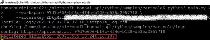

Note : With the following CLI command, you can also see the list of session id for running simulators.

bonsai simulator unmanaged list

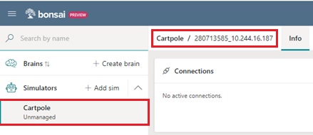
In Bonsai UI (workspace UI) on cloud, the connected instance will be shown as follows.
As you can see below, the simulator session id is also displayed on this screen.

Brain and Inkling (Basic)

Now let’s create a machine teaching model, called a brain.

To start to create a brain, press “Create brain” button in Bonsai UI.
In this example, please select “Empty brain” as follows, because we’ll build a brain from scratch.

Note : You can delete a brain in brain info window.

Now this will be a main part for working with Project Bonsai.
Each machine teaching is managed in a brain object, and the specification for machine teaching is defined with domain specific language, named “Inkling”.

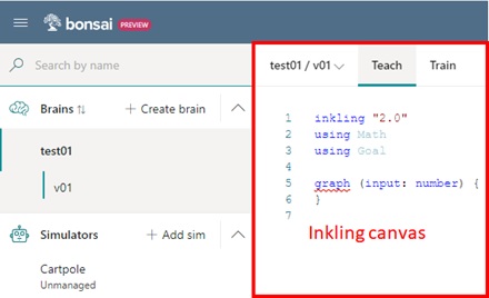
To demystify Inkling descriptions, first we start with minimal Inkling definition as follows.

inkling "2.0"using Mathusing Goal# Statetype SimState {  cart_position: number,  cart_velocity: number,  pole_angle: number,  pole_angular_velocity: number,  pole_center_position: number,   pole_center_velocity: number,  target_pole_position: number,  cart_mass: number,  pole_mass: number,  pole_length: number,}# Actiontype Action {  command: number<-1..1>}graph (input: SimState): Action {  concept BalancePole(input): Action {curriculum {  source simulator (Action: Action): SimState {  }  training {EpisodeIterationLimit: 200,NoProgressIterationLimit: 10000,  }  goal (SimState: SimState) {avoid FallOver:  Math.Abs(SimState.pole_angle) in Goal.RangeAbove((12 * 2 * Math.Pi) / 360)avoid OutOfRange:  Math.Abs(SimState.cart_position) in Goal.RangeAbove(1.0)  }}  }}const SimulatorVisualizer = "/cartpoleviz/"

As I mentioned above (see “Reinforcement Learning and CartPole example”), CartPole has an action and state, which is a numeric value and a composite value (including cart position, pole angle, …) respectively. These types are defined in above SimState and Action.
By specifying number<-1..1> in Action, it means that the range of action is between -1 and 1 (inclusive).

The concept keyword defines a component that must be learned. With this BalancePole concept, it defines a single machine teaching (training).

In this concept section, EpisodeIterationLimit keyword defines the maximum number of iterations per a single episode. (In this case, 200 iterations / episode.)
By NoProgressIterationLimit keyword, the training will be completed when it learns well enough and no progress in 10,000 iterations.

The goal setting will be a critical task for engineers.
In practice, the engineers want to set a variety of goals – such as, preventing from some situation, reaching to some threshold, resolving some problem, or keeping some state. With Project Bonsai, the engineers don’t necessarily have skills for reinforcement learning, and free to set intuitive goals by Inkling.
Bonsai framework will then resolve these settings defined by engineers and take into training actions.

In this example,

• When the absolute value of pole angle exceeds , the episode is considered as failure and is then terminated.
• When the absolute value of cart position exceeds 1.0, the episode is considered as failure and is then terminated.

Then a brain will learn not to go into these failure states in machine teaching.

For instance, if your goal is to minimize |target_pole_position - cart_position|, you can describe a goal as follows.

minimize DistToTarget:  Math.Abs(SimState.target_pole_position - SimState.cart_position) in Goal.RangeBelow(0)

Unlike regular reinforcement learning, you don’t need to explicitly declare data scientific settings – such as, selecting RL algorithms/models/distributions, setting a variety of hyper-parameters, and designing rewards, etc. (RL algorithm will be automatically determined by problem settings in Bonsai framework.)

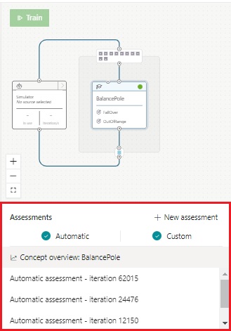
In Bonsai UI, the graph of this Inkling will be shown as follows.
As you can see below, here a graph contains a single primitive concept for machine teaching. (Later I’ll discuss about multiple concepts.)

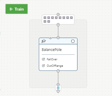
The SimulatorVisualizer is specifying a simulator’s visualizer. While it’s running training or assessment, the visualizer will receive states and show visuals in real-time.
In this example, built-in CartPole visualizer is used in Inkling. (See below.)

If you are a simulation provider, you can integrate your own simulator as Bonsai visualizer plugin. Here I don’t go so far, but please refer here for creating custom visualizer. (It can be simply written by JavaScript with event handlers.)

Inkling – Episode Initialization

In this example, I don’t specify any configuration to initialize each episode, and it will then always pass None for episode’s initialization. As a result, both initial_cart_position and target_pole_position are always initialized as 0 in training. (See below code for simulator’s reset. The default value for these parameters equals to 0.)

sim/cartpole.py

...class CartPole:  ...  def reset(self,cart_mass: float = DEFAULT_CART_MASS,pole_mass: float = DEFAULT_POLE_MASS,pole_length: float = DEFAULT_POLE_LENGTH,initial_cart_position: float = 0,initial_cart_velocity: float = 0,initial_pole_angle: float = 0,initial_angular_velocity: float = 0,target_pole_position: float = 0,  ):...

To train more intelligent, it will be better to pass randomized values for initial_cart_position and target_pole_position in each episode.
For doing this, define the following initialization configuration (init config) SimConfig and configure episode’s initialization with lesson keyword as follows.

inkling "2.0"using Mathusing Goal# Statetype SimState {  cart_position: number,  cart_velocity: number,  pole_angle: number,  pole_angular_velocity: number,  pole_center_position: number,   pole_center_velocity: number,  target_pole_position: number,  cart_mass: number,  pole_mass: number,  pole_length: number,}# Actiontype Action {  command: number<-1..1>}# Configuration variablestype SimConfig {  cart_mass: number,  pole_mass: number,  pole_length: number,  initial_cart_position: number<-1.0 .. 1.0>,  initial_cart_velocity: number,  initial_pole_angle: number,  initial_angular_velocity: number,  target_pole_position: number<-1.0 .. 1.0>,}graph (input: SimState): Action {  concept BalancePole(input): Action {curriculum {  source simulator (Action: Action, Config: SimConfig): SimState {  }  training {EpisodeIterationLimit: 200,NoProgressIterationLimit: 10000,  }  goal (SimState: SimState) {avoid FallOver:  Math.Abs(SimState.pole_angle) in Goal.RangeAbove((12 * 2 * Math.Pi) / 360)avoid OutOfRange:  Math.Abs(SimState.cart_position) in Goal.RangeAbove(1.0)  }  lesson TestLesson {scenario {  initial_cart_position: number<-1.0 .. 1.0>,  target_pole_position: number<-1.0 .. 1.0>}  }}  }}const SimulatorVisualizer = "/cartpoleviz/"

By this setting, Bonsai will set randomized value between -1.0 and 1.0 (inclusive) for both initial_cart_position and target_pole_position in each episode’s initialization.
These variables can then be passed as simulator’s initialization in custom code as follows.

main.py

from sim import cartpole...self.simulator = cartpole.CartPole()...def episode_start(self, config: Dict = None) -> None:  if config is None:config = default_config  self.config = config  self.simulator.reset(**config)if ... :  ...elif event.type == "EpisodeStart":  print(event.episode_start.config)  sim.episode_start(event.episode_start.config)...

Depending on simulators, engineers can customize a lot of simulator’s behaviors.

Inkling – Multiple Concepts

In more practical machine teaching, several scenarios might be related and combined.
For instance, suppose, some autonomous system would differently work in high temperature and low temperature, and it might get better performance when each situation is separately trained and finally combined.
By modifying above CartPole example, let me show you a simple example.

The following Inkling description defines 2 concepts – GoLeft and GoRight.

• GoLeft : The episode will start with 0 <= initial_cart_position <= 1.0 (i.e, right-side position) and the agent will learn to go left.
• GoRight : The episode will start with -1.0 <= initial_cart_position <= 0 (i.e, left-side position) and the agent will learn to go right.

inkling "2.0"using Mathusing Goal# Statetype SimState {  cart_position: number,  cart_velocity: number,  pole_angle: number,  pole_angular_velocity: number,  pole_center_position: number,  pole_center_velocity: number,  target_pole_position: number,  cart_mass: number,  pole_mass: number,  pole_length: number,}# Actiontype Action {  command: number<-1 .. 1>}# Configuration variablestype SimConfig {  cart_mass: number,  pole_mass: number,  pole_length: number,  initial_cart_position: number<-1.0 .. 1.0>,  initial_cart_velocity: number,  initial_pole_angle: number,  initial_angular_velocity: number,  target_pole_position: number<-1.0 .. 1.0>,}graph (input: SimState): Action {  concept GoLeft(input): Action {curriculum {  source simulator (Action: Action, Config: SimConfig): SimState {  }  training {EpisodeIterationLimit: 200,NoProgressIterationLimit: 10000,  }  goal (SimState: SimState) {avoid FallOver:  Math.Abs(SimState.pole_angle)  in Goal.RangeAbove((12 * 2 * Math.Pi) / 360)avoid OutOfRange:  Math.Abs(SimState.cart_position)  in Goal.RangeAbove(1.0)  }  lesson TestLesson {scenario {  initial_cart_position: number<0 .. 1.0>,  target_pole_position: 0}  }}  }  concept GoRight(input): Action {curriculum {  source simulator (Action: Action, Config: SimConfig): SimState {  }  training {EpisodeIterationLimit: 200,NoProgressIterationLimit: 10000,  }  goal (SimState: SimState) {avoid FallOver:  Math.Abs(SimState.pole_angle)  in Goal.RangeAbove((12 * 2 * Math.Pi) / 360)avoid OutOfRange:  Math.Abs(SimState.cart_position)  in Goal.RangeAbove(1.0)  }  lesson TestLesson {scenario {  initial_cart_position: number<-1.0 .. 0>,  target_pole_position: 0}  }}  }  output concept PickOne(input): Action {select GoLeftselect GoRightcurriculum {  source simulator (Action: Action, Config: SimConfig): SimState {  }  training {EpisodeIterationLimit: 200,NoProgressIterationLimit: 10000,  }  goal (SimState: SimState) {avoid FallOver:  Math.Abs(SimState.pole_angle)  in Goal.RangeAbove((12 * 2 * Math.Pi) / 360)avoid OutOfRange:  Math.Abs(SimState.cart_position)  in Goal.RangeAbove(1.0)  }  lesson TestLesson {scenario {  initial_cart_position: number<-1.0 .. 1.0>,  target_pole_position: 0}  }}  }}const SimulatorVisualizer = "/cartpoleviz/"

Note : When there exist more than one concept, you should explicitly specify which concept generates the brain’s output by adding output keyword as above.

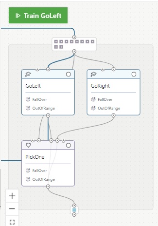
In this training execution, each concept is separately trained (i.e, train 2 models) and after the training of these 2 concepts, you can then finally train the combined PickOne concept. (Total 3 trainings are executed separately.)

If you want to pick up one (GoLeft or GoRight) with some specific rules, you can also build a simple rule-based function, using a programmed concept.
For instance, the following Inkling will pick up GoLeft action when target_pole_position < 0 and GoRight otherwise.

inkling "2.0"using Mathusing Goal# Statetype SimState {  cart_position: number,  cart_velocity: number,  pole_angle: number,  pole_angular_velocity: number,  pole_center_position: number,  pole_center_velocity: number,  target_pole_position: number,  cart_mass: number,  pole_mass: number,  pole_length: number,}# Actiontype Action {  command: number<-1 .. 1>}# Configuration variablestype SimConfig {  cart_mass: number,  pole_mass: number,  pole_length: number,  initial_cart_position: number<-1.0 .. 1.0>,  initial_cart_velocity: number,  initial_pole_angle: number,  initial_angular_velocity: number,  target_pole_position: number<-1.0 .. 1.0>,}graph (input: SimState): Action {  concept GoLeft(input): Action {curriculum {  source simulator (Action: Action, Config: SimConfig): SimState {  }  training {EpisodeIterationLimit: 200,NoProgressIterationLimit: 10000,  }  goal (SimState: SimState) {avoid FallOver:  Math.Abs(SimState.pole_angle)  in Goal.RangeAbove((12 * 2 * Math.Pi) / 360)avoid OutOfRange:  Math.Abs(SimState.cart_position)  in Goal.RangeAbove(1.0)  }  lesson TestLesson {scenario {  initial_cart_position: number<0 .. 1.0>,  target_pole_position: 0}  }}  }  concept GoRight(input): Action {curriculum {  source simulator (Action: Action, Config: SimConfig): SimState {  }  training {EpisodeIterationLimit: 200,NoProgressIterationLimit: 10000,  }  goal (SimState: SimState) {avoid FallOver:  Math.Abs(SimState.pole_angle)  in Goal.RangeAbove((12 * 2 * Math.Pi) / 360)avoid OutOfRange:  Math.Abs(SimState.cart_position)  in Goal.RangeAbove(1.0)  }  lesson TestLesson {scenario {  initial_cart_position: number<-1.0 .. 0>,  target_pole_position: 0}  }}  }  output concept PickOne(input, GoLeft, GoRight): Action {programmed function (state: SimState, action_left: Action, action_right: Action): Action {  # Pick action programmatically  if state.target_pole_position < 0 {return action_left  }  return action_right}  }}const SimulatorVisualizer = "/cartpoleviz/"

In this CartPole example, it will be useless to separately train multiple concepts (because the problem is very simple), but, depending on the difficulty of problems, this approach will be helpful and engineers can easily design these advanced machine teaching with Inkling.

Inkling – Advanced Settings by AI Specialists

If needed, data scientists can also assist by adding AI specific definitions in Inkling.

For instance, the following Inkling defines a reward score in each step, as a data scientist does in regular reinforcement learning.

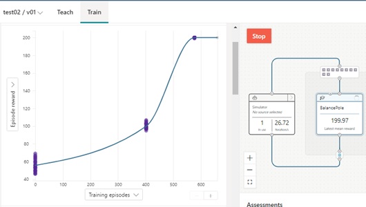
inkling "2.0"using Mathusing Goal# Statetype SimState {  cart_position: number,  cart_velocity: number,  pole_angle: number,  pole_angular_velocity: number,  pole_center_position: number,   pole_center_velocity: number,  target_pole_position: number,  cart_mass: number,  pole_mass: number,  pole_length: number,}# Actiontype Action {  command: number<-1..1>}# Configuration variablestype SimConfig {  cart_mass: number,  pole_mass: number,  pole_length: number,  initial_cart_position: number<-1.0 .. 1.0>,  initial_cart_velocity: number,  initial_pole_angle: number,  initial_angular_velocity: number,  target_pole_position: number<-1.0 .. 1.0>,}function GetReward(state: SimState) {  if Math.Abs(state.target_pole_position - state.cart_position) < 0.2 {return 1.0  }  return -0.01}graph (input: SimState): Action {  concept BalancePole(input): Action {curriculum {  source simulator (Action: Action, Config: SimConfig): SimState {  }  training {EpisodeIterationLimit: 200,NoProgressIterationLimit: 10000,  }  reward GetReward  terminal function (state: SimState) {if Math.Abs(state.pole_angle) > (12 * 2 * Math.Pi) / 360 {  return 1}if Math.Abs(state.cart_position) > 1.0 {  return 1}return 0  }}  }}const SimulatorVisualizer = "/cartpoleviz/"

When you run this training, you will be able to see how episode reward’s mean is improved as follows.
This reward transition (curve) will be more familiar for most data scientists.

Note : In reward-based training, you can complete training when the cumulative reward meets or exceeds some threshold value. (See LessonRewardThreshold in Inkling reference.)

You can also explicitly specify RL algorithms (currently, APEX, PPO and SAC are supported), and tune hyper-parameters for a selected algorithm. (See here for details.)

...graph (input: SimState): Action {  concept BalancePole(input): Action {curriculum {  source simulator (Action: Action, Config: SimConfig): SimState {  }  algorithm {Algorithm: "SAC",QHiddenLayers: [  {Size: 256,Activation: "relu"  },  {Size: 256,Activation: "relu"  }],PolicyHiddenLayers: [  {Size: 256,Activation: "relu"  },  {Size: 256,Activation: "relu"  }],  }  ...}  }}...

Project Bonsai also supports the imported skill (ML model which is trained outside) using a imported concept.
To use imported concepts, import the model and use import keyword as follows. Make sure that the input state and output in the imported model should have the same dimension as type definitions in Inkling it maps to.

concept ImportedConcept(input): Action {  import {Model: "HoneyHouse"}}

The following is the supported formats for imported models. (See here for details.)

• Open Neural Network Exchange (ONNX) – recommended using PyTorch
• TensorFlow Frozen GraphDef
• TensorFlow Saved Model

For example, screen state by 2D or 3D array of numbers can be processed by an imported convolution (CNN) model which is trained outside.

Note : Image input is not currently supported in the imported model. (Use the array of numbers.)

Run Training

After you have built Inkling, now let’s start to train your brain.

Before you start training, please configure the unmanaged simulator’s connection as follows. (In the following command, “BalancePole” should be a concept name in Inkling, and “Cartpole” should be a simulator name.)
When you use a managed simulator (later I’ll explain about managed simulator), this won’t be needed.

bonsai simulator unmanaged connect \  -b {BRAIN-NAME} \  -a Train \  -c BalancePole \  --simulator-name Cartpole

To start training, click “Train” button and select a registered simulator (in this example, unmanaged simulator “Cartpole”).

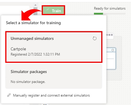
Note : When a brain has multiple concepts, select a concept and then click the train button.

Once the training is started, Bonsai will reset an episode, step over and over, and terminate an episode. As I have mentioned above (see “Reinforcement Learning and CartPole example”), the episode will be repeated and the model will be trained.

Our custom simulator program (main.py) will receive Bonsai events and proceed an simulator depending on that event. And the result’s state (the following SimulatorState) is passed into a brain by the following client.session.advance() and the next action (the following event.episode_step.action) is extracted from Bonsai event. This iteration will be repeated.
As you can see below, these can be performed by Python Bonsai API.

main.py

...from microsoft_bonsai_api.simulator.client import BonsaiClient, BonsaiClientConfigfrom microsoft_bonsai_api.simulator.generated.models import (  SimulatorInterface,  SimulatorState,  SimulatorSessionResponse,)...def main(...)  ...  config_client = BonsaiClientConfig()  client = BonsaiClient(config_client)  ...  try:while True:  sim_state = SimulatorState(sequence_id=sequence_id, state=sim.get_state(), halted=sim.halted(),  )  try:event = client.session.advance(  workspace_name=config_client.workspace,  session_id=registered_session.session_id,  body=sim_state,)sequence_id = event.sequence_idprint(  "[{}] Last Event: {}".format(time.strftime("%H:%M:%S"), event.type))  except HttpResponseError as ex:...  except Exception as err:...  if event.type == "Idle":...  elif event.type == "EpisodeStart":...  elif event.type == "EpisodeStep":...sim.episode_step(event.episode_step.action)...  elif event.type == "EpisodeFinish":...  elif event.type == "Unregister":...  else:...

In Bonsai UI, you can see that the simulator visualizer is updated in real-time. (Here I have trained a brain with above minimal Inkling configuration.)

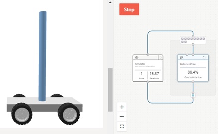
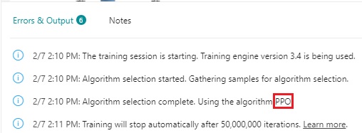
As you can see in the output on Bonsai UI, PPO (Proximal Policy Optimization) is automatically selected as RL algorithm in this example. Here I don’t go so far, but please see here (my GitHub repo) for PPO algorithm.

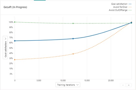
You can also see the curve of goal satisfaction (in this example, FallOver and OutOfRange) in Bonsai UI. As you can see below, OutOfRange objective is already satisfied from the beginning of training, but FallOver objective is learned and improved by machine teaching.

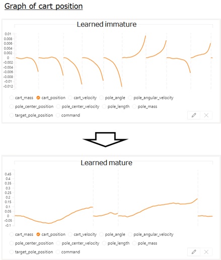
You can easily see intuitive insights by a variety of graph (visualization) and metrics on Bonsai UI.
For instance, the following chart will show you how the motion of cart position is improved during training.

Run Simulator Package on Cloud (Managed Simulator)

Up until now, we were running an unmanaged local simulator on Ubuntu VM.
Now let’s build a simulator package and run on managed cloud environments.

By running az command as follows, build this Python program as a simulator package (i.e, a docker image) and upload into your Azure container registry (ACR) in Bonsai workspace.

Note : The following {ACR-REGISTRY-NAME} in command should be a container registry name in Bonsai resource.

# Login to your subscriptionaz loginaz account set --subscription {SUBSCRIPTION-ID}# Build image and upload to ACRaz acr build --image carts_and_poles:v1 --file Dockerfile --registry {ACR-REGISTRY-NAME} .

Dockerfile

# this is one of the cached base images available for ACIFROM python:3.7.4# Install libraries and dependenciesRUN apt-get update && \  apt-get install -y --no-install-recommends \  build-essential \  cmake \  zlib1g-dev \  swig# Set up the simulatorWORKDIR /src# Copy simulator files to /srcCOPY . /src# Install simulator dependenciesRUN pip3 install -r requirements.txt# This will be the command to run the simulatorCMD ["python3", "main.py"]# This command runs the simulator with a 3s delay + uniform variance +/-1#CMD ["python3", "main.py", "--sim-speed", "3", "--sim-speed-variance", "1"]

Now it’s ready for running your own managed simulator.
In Bonsai UI, select “Add sim” button to add the registered simulator into workspace.

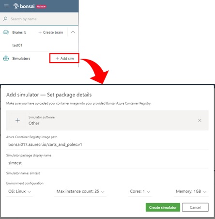
Create and configure a brain (with Inkling) as usual.
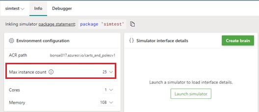
Then, set the instance count as follows and click “Train” to start training.

In training, all instances are automatically launched in Azure Container Instance (ACI) and connected to a Bonsai brain. (When the training is completed, all running instances are automatically terminated.)
All these tasks are managed by Bonsai framework.

The training will robustly scale to multiple instances and the brain can then be quickly learned.
Let’s compare the training speed with unmanaged simulator !

Logging

Project Bonsai is integrated with log analytics in Microsoft Azure.

Note : To gather logs in unmanaged simulator, please run the following command after the simulator has connected. When using a managed simulator, you don’t need to run as follows. (Workloads on managed simulator is automatically logged.)

bonsai brain version start-logging \  --name {BRAIN-NAME} \  --session-id {SESSION-ID}

When you stop logging, run as follows.

bonsai brain version stop-logging \  --name {BRAIN-NAME} \  --session-id {SESSION-ID}

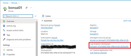
Go to log analytics workspace by clicking the following link in Bonsai resource.

Now you can run Kusto query (KQL) in log analytics workspace. Select “Logs” menu (in “General” section) in log analytics workspace and run Kusto query as you like.
For instance, run the following query, when you monitor the reward in training.

EpisodeLog_CL| where BrainName_s == '{BRAIN-NAME}' and BrainVersion_d == '1'| join kind=inner (IterationLog_CL) on EpisodeId_g| project  EpisodeId = EpisodeId_g,  IterationIndex = IterationIndex_d,  Timestamp = Timestamp_t,  Reward = Reward_d| order by EpisodeId asc, IterationIndex asc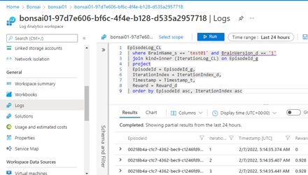

Note : In logs, you can see the cumulative rewards (CumulativeReward_d) or goal metrics, and you can then summarize how it learned.

The query results can be saved as CSV and can then be analyzed with external program, such as, Excel, Python code, etc.

Assessment

Once you have a trained brain, you can run assessment by specifying an array of one or more entries that represent init config values.
(See above “Inkling – Episode Initialization” for init config. For assessment, please define init config in Inkling.)

For instance, the following assessment configuration will run 10 episodes with the following init config values for each episode.

{  "version": "1.0.0",  "context": {},  "episodeConfigurations": [{  "initial_cart_position": -0.46438068439203906,  "target_pole_position": 0.33269671353395547},{  "initial_cart_position": -0.15986215549005833,  "target_pole_position": 0.11657382544776951},{  "initial_cart_position": -0.3898316216812683,  "target_pole_position": 0.050723439591823793},{  "initial_cart_position": -0.28539041883886107,  "target_pole_position": 0.15521480035502855},{  "initial_cart_position": -0.4214730833940563,  "target_pole_position": 0.08478363140971834},{  "initial_cart_position": -0.01541274895886302,  "target_pole_position": 0.16281345490933996},{  "initial_cart_position": -0.38172259372996675,  "target_pole_position": 0.4023297210629143},{  "initial_cart_position": -0.2602582844411645,  "target_pole_position": 0.2838278501449083},{  "initial_cart_position": -0.15073398658203907,  "target_pole_position": 0.44139050005368063},{  "initial_cart_position": -0.1920145268964113,  "target_pole_position": 0.4627648928745359}  ]}

Note : Bonsai UI can also assist to generate an assessment configuration. To be honest, the above configuration is also auto-generated by the following setting.

Bonsai also supports automatic assessment, which is auto-configured assessment.

Note : When you run assessment on unmanaged simulator, please connect with the following Assess action’s setting.

bonsai simulator unmanaged connect \  -b {BRAIN-NAME} \  -a Assess \  -c BalancePole \  --simulator-name Cartpole

After the assessment run has completed, you can view a variety of metrics in assessment UI. (See below.)
In this example, you will find that the result is insufficient (see below), because I have trained a model with initial_cart_position = target_pole_position = 0 (default value).

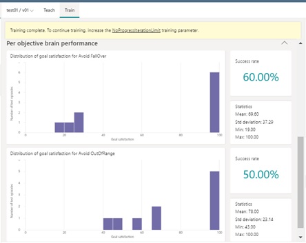
If the result is not acceptable, modify Inkling configuration and re-generate (re-train) a model. It will automatically generate a new version of brain, and you will then repeat assessments again. (Please repeat this cycle to satisfy your goal.)

Note : You can also query the assessment data with log analytics. (Each log entry has AssessmentName_s field when the episode is run on assessment.)

Deploy Trained Model

Once you have passed assessments, finally proceed to deploy a trained model into production.

Each version of brain maintains its own trained model, and you can export a brain as docker image by clicking “Export brain”. (See below.)

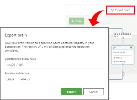
Your exported image is then stored in a container registry (ACR) in Bonsai workspace, and you can run image anywhere, such as, AKS (Kubernetes), ACI, Web App for Containers, or IoT devices.

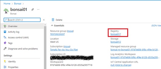
Note : The repository name in ACR will be same as a Bonsai workspace id.

For instance, the following command will download and run a container image locally.

# Connect to ACRaz loginaz acr login --name {ACR-NAME}# Pull image from ACRdocker pull \  {SERVER-NAME}.azurecr.io/{REPOSITORY-NAME}/{IMAGE-NAME}:{TAG-NAME}# Run container in localdocker run -d -p 5000:5000 \  {SERVER-NAME}.azurecr.io/{REPOSITORY-NAME}/{IMAGE-NAME}:{TAG-NAME}

With port 5000, you can submit HTTP request for a trained brain as follows.
In the following request, 116de3e7-b8c9-4cfa-951d-d10f9fcc6be4 must be a uuid for identifying a client. (You should then create your own uuid.)

HTTP request

http://localhost:5000/v2/clients/116de3e7-b8c9-4cfa-951d-d10f9fcc6be4/predictContent-Type: application/json{  "state": {"cart_position": 0.5,"cart_velocity": 1.5,"pole_angle": 0.75,"pole_angular_velocity": 0.1,"pole_center_position": 0,"pole_center_velocity": 0,"target_pole_position": 0,"cart_mass": 0.31,"pole_mass": 0.055,"pole_length": 0.4  }}

HTTP response

HTTP/1.1 200 OKContent-Type: application/json{  "clientId": "116de3e7-b8c9-4cfa-951d-d10f9fcc6be4",  "concepts": {"BalancePole": {  "action": {"command": 0.3575190007686615  }}  }}

Note : You can see API specification at http://localhost:5000/swagger.html

The model format used in the exported image (v2) is TensorFlow Lite, which is light-weight model applicable for edge devices.

In this post, I have introduced the architecture of Bonsai for engineers.
For software vendors, the simulation platforms can immediately get benefit of proven AI framework, by integrating with Bonsai.
Bonsai currently works with a lot of software vendors and now supports a variety of commercial simulation platforms. (Find simulation platforms in “Bonsai simulation partners“.)