As you can see in 3rd party’s benchmarking results for Test-H and Test-DS* (see here), the dedicated SQL pools in Azure Synapse Analytics (formerly, Azure SQL Data Warehouse) outperforms compared with other analytics database, such as, BigQuery, Redshift, and Snowflake.
However, to take this advantage of better performance and cost-effectiveness in such a limitless architecture, MPP (massively parallel processing), you should consider several things, such as, partitioning, indexing, caching, so on and so forth.

In my several posts in series, I’ll show you well-known techniques (tutorials) in layouts and design to optimize performance in Azure Synapse Analytics SQL dedicated pools using real code and examples.

Synapse Analytics : Designing for Performance – Table of Contents

1. Optimize for Distributions (this post)
2. Choose Right Index and Partition
3. How Statistics and Cache Works

In this post, we see distribution strategies.

Note : Throughout my posts in series, I will often use World Wide Importer samples. If you follow my writing, please see here and import sample data into your own pool.

Replication Strategy (Optimize Broadcast Data Movement)

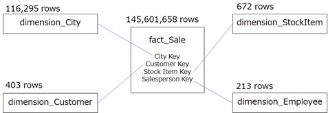
First, let me assume the following tables for both fact table (transaction table) and surrounding dimension tables, i.e, which has the structure, so-called “star schema”.

When you create a table without specifying a distribution strategy as follows, Synapse Analytics will create a table with round-robin fashion for distribution strategy. That is, each rows will be distributed in each databases (it’s totally 60 databases in a single pool) in round-robin fashion.

CREATE TABLE [wwi].[dimension_City](   [City Key] int NOT NULL,  [WWI City ID] int NOT NULL,  [City] nvarchar(50) NOT NULL,  ...)

This round-robin fashion table is optimal for loading large raw data, but not optimal for querying in most cases.

Now let’s try to run the following query for this round-robin fashion table.

SELECT TOP(100) s.[Sale Key], c.[City]FROM [wwi].[fact_Sale] s LEFT JOIN [wwi].[dimension_City] c ON s.[City Key] = c.[City Key]

In order to see the execution plan (see how optimal plan is determined and the query will be executed) for this query, please run the following script by simply adding EXPLAIN clause at the beginning.

EXPLAINSELECT TOP(100) s.[Sale Key], c.[City]FROM [wwi].[fact_Sale] s LEFT JOIN [wwi].[dimension_City] c ON s.[City Key] = c.[City Key]

output

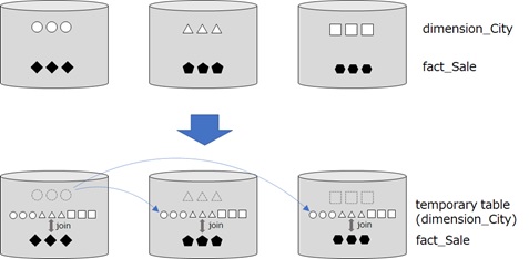
<?xml version="1.0" encoding="utf-8"?><dsql_query number_nodes="1" number_distributions="60" number_distributions_per_node="60">  <sql>SELECT TOP(100) s.[Sale Key], c.[City]FROM [wwi].[fact_Sale] s LEFT JOIN [wwi].[dimension_City] c ON s.[City Key] = c.[City Key]</sql>  <dsql_operations total_cost="2902.7232" total_number_operations="5"><dsql_operation operation_type="RND_ID">  <identifier>TEMP_ID_3</identifier></dsql_operation><dsql_operation operation_type="ON">  <location permanent="false" distribution="AllComputeNodes" />  <sql_operations><sql_operation type="statement">CREATE TABLE [qtabledb].[dbo].[TEMP_ID_3] ([City Key] INT NOT NULL, [City] NVARCHAR(50) COLLATE SQL_Latin1_General_CP1_CI_AS NOT NULL ) WITH(DISTRIBUTED_MOVE_FILE='');</sql_operation>  </sql_operations></dsql_operation><dsql_operation operation_type="BROADCAST_MOVE">  <operation_cost cost="2902.7232" accumulative_cost="2902.7232" average_rowsize="104" output_rows="116295" GroupNumber="4" />  <source_statement>SELECT [T1_1].[City Key] AS [City Key], [T1_1].[City] AS [City] FROM [WWI_test01].[wwi].[dimension_City] AS T1_1OPTION (MAXDOP 1, MIN_GRANT_PERCENT = [MIN_GRANT], DISTRIBUTED_MOVE(N''))</source_statement>  <destination_table>[TEMP_ID_3]</destination_table></dsql_operation><dsql_operation operation_type="RETURN">  <location distribution="AllDistributions" />  <select>SELECT [T1_1].[Sale Key] AS [Sale Key], [T1_1].[City] AS [City] FROM (SELECT TOP (CAST ((100) AS BIGINT)) [T2_2].[Sale Key] AS [Sale Key], [T2_1].[City] AS [City] FROM [qtabledb].[dbo].[TEMP_ID_3] AS T2_1 RIGHT OUTER JOIN[WWI_test01].[wwi].[fact_Sale] AS T2_2ON ([T2_2].[City Key] = [T2_1].[City Key])) AS T1_1OPTION (MAXDOP 1, MIN_GRANT_PERCENT = [MIN_GRANT])</select></dsql_operation><dsql_operation operation_type="ON">  <location permanent="false" distribution="AllComputeNodes" />  <sql_operations><sql_operation type="statement">DROP TABLE [qtabledb].[dbo].[TEMP_ID_3]</sql_operation>  </sql_operations></dsql_operation>  </dsql_operations></dsql_query>

By above BROADCAST_MOVE operation, the rows in dimension_City table are all copied in a temporary table (called TEMP_ID_3) on all distributed database. (See below.)
Since the size of dimension_City is small, then all rows in this table is duplicated in all database before joining. This time, we join only 2 tables, however, if a lot of tables are needed to join, this data movement will become large overhead for query execution.
A temporary table will be dropped after the query is completed. Then this overhead might also be happened in the next same query.

Note : In order to get the recommendations to optimize performance with query plan, you can use EXPLAIN WITH_RECOMMENDATIONS statement instead.

Note : By using sys.dm_pdw_request_steps table (dynamic management view, DMV), you can see how the operation is actually executed and how long it took as follows, after you’ve run the query.

SELECT request_id AS req, step_index AS i, operation_type, distribution_type, start_time, end_time, commandFROM sys.dm_pdw_request_stepsWHERE request_id = 'QID303'

reqi operation_type distribution_type start_time  end_timecommand---------------------------------------------------------------------------------------------------------------------QID303 0 RandomIDOperation  Unspecified   2020-10-07T00:52:27.8230000 2020-10-07T00:52:27.8230000 TEMP_ID_3QID303 1 OnOperationAllComputeNodes   2020-10-07T00:52:27.8230000 2020-10-07T00:52:27.8700000 CREATE TABLE [qtabledb].[dbo].[TEMP_ID_3] ...QID303 2 BroadcastMoveOperation AllDistributions  2020-10-07T00:52:27.8700000 2020-10-07T00:52:27.9930000 SELECT [T1_1].[City Key] ...QID303 3 ReturnOperationAllDistributions  2020-10-07T00:52:27.9930000 2020-10-07T00:52:29.8830000 SELECT [T1_1].[Sale Key] AS [Sale Key] ...QID303 4 OnOperationAllComputeNodes   2020-10-07T00:52:29.8830000 2020-10-07T00:52:29.8830000 DROP TABLE [qtabledb].[dbo].[TEMP_ID_3]

You can also monitor the execution using other DMVs. (In this post, I don’t go so far about DMV.)
For instance, you can view how many rows are moved in data movement service (DMS) using sys.dm_pdw_dms_workers as follows.

SELECT distribution_id, type, rows_processed FROM sys.dm_pdw_dms_workersWHERE request_id = 'QID1765' AND step_index = 11;

Note : Adding FORCE ORDER hint can force the query optimizer to apply the order of joins to be executed as writing.

Note : For monitoring tempdb usage in query, see here.

In order to ensure that all rows should be copied and persisted in all distributed database explicitly, use REPLICA strategy for dimension tables, instead of using ROUND_ROBIN. (See below.)

DROP TABLE [wwi].[dimension_City];GOCREATE TABLE [wwi].[dimension_City]...WITH(   DISTRIBUTION = REPLICATE,  CLUSTERED COLUMNSTORE INDEX)GO

Now you will see that the query is planed without data movement.

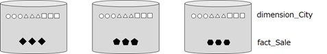
EXPLAINSELECT TOP(100) s.[Sale Key], c.[City]FROM [wwi].[fact_Sale] s LEFT JOIN [wwi].[dimension_City] c ON s.[City Key] = c.[City Key]

<?xml version="1.0" encoding="utf-8"?><dsql_query number_nodes="1" number_distributions="60" number_distributions_per_node="60">  <sql>SELECT TOP(100) s.[Sale Key], c.[City]FROM [wwi].[fact_Sale] s LEFT JOIN [wwi].[dimension_City] c ON s.[City Key] = c.[City Key]</sql>  <dsql_operations total_cost="0" total_number_operations="1"><dsql_operation operation_type="RETURN">  <location distribution="AllDistributions" />  <select>SELECT [T1_1].[Sale Key] AS [Sale Key], [T1_1].[City] AS [City] FROM (SELECT TOP (CAST ((100) AS BIGINT)) [T2_2].[Sale Key] AS [Sale Key], [T2_1].[City] AS [City] FROM [WWI_test01].[wwi].[dimension_City] AS T2_1 RIGHT OUTER JOIN[WWI_test01].[wwi].[fact_Sale] AS T2_2ON ([T2_2].[City Key] = [T2_1].[City Key])) AS T1_1OPTION (MAXDOP 1)</select></dsql_operation>  </dsql_operations></dsql_query>

In REPLICA strategy, all rows in a table (dimension_City table in our case) are copied in all distributed database in the first query running. (Even when you run EXPLAIN statement, this will happen.)
Once copied tables are generated in all distributed database, these tables will be reused for the following various queries. (Unlike a temporary table, this replicated tables will not be dropped after the query is completed.)

In replicate table, the copied tables and corresponding indexes in all distributions will be generated only once in the first query running. For this activity, it will be better to run query to ensure table’s copy, once the replicate table is created and all data is loaded.

Note : When you update rows in this table (with REPLICA strategy), the replicated cache is invalidated. Then all rows are copied again into all distributions in the next query.
Hence, please avoid frequently updating the replication table.

Hash Distribution (Avoid Shuffle Data Movement)

Now let’s see another example.
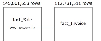
In this example, we join fact_Sale table and fact_Invoice table as follows. As you can see, both are large tables unlike above star schema sample.

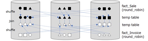
If you use default round-robin strategy for these tables, a query plan for this join will become as follows.

EXPLAINSELECT TOP(100) s.[Unit Price], s.[Quantity], i.[Customer Key]FROM [wwi].[fact_Sale] s LEFT JOIN [wwi].[fact_Invoice] i ON s.[WWI Invoice ID] = i.[WWI Invoice ID]

<?xml version="1.0" encoding="utf-8"?><dsql_query number_nodes="1" number_distributions="60" number_distributions_per_node="60">  <sql>SELECT TOP(100) s.[Unit Price], s.[Quantity], i.[Customer Key]FROM [wwi].[fact_Sale] s LEFT JOIN [wwi].[fact_Invoice] i ON s.[WWI Invoice ID] = i.[WWI Invoice ID]</sql>  <dsql_operations total_cost="11499.3712" total_number_operations="9"><dsql_operation operation_type="RND_ID">  <identifier>TEMP_ID_8</identifier></dsql_operation><dsql_operation operation_type="ON">  <location permanent="false" distribution="AllDistributions" />  <sql_operations><sql_operation type="statement">CREATE TABLE [qtabledb].[dbo].[TEMP_ID_8] ([WWI Invoice ID] INT NOT NULL, [Customer Key] INT ) WITH(DISTRIBUTED_MOVE_FILE='');</sql_operation>  </sql_operations></dsql_operation><dsql_operation operation_type="SHUFFLE_MOVE">  <operation_cost cost="1598.4352" accumulative_cost="1598.4352" average_rowsize="8" output_rows="49951100" GroupNumber="4" />  <source_statement>SELECT [T1_1].[WWI Invoice ID] AS [WWI Invoice ID], [T1_1].[Customer Key] AS [Customer Key] FROM [WWI_test01].[wwi].[fact_Invoice] AS T1_1OPTION (MAXDOP 1, MIN_GRANT_PERCENT = [MIN_GRANT], DISTRIBUTED_MOVE(N''))</source_statement>  <destination_table>[TEMP_ID_8]</destination_table>  <shuffle_columns>WWI Invoice ID;</shuffle_columns></dsql_operation><dsql_operation operation_type="RND_ID">  <identifier>TEMP_ID_9</identifier></dsql_operation><dsql_operation operation_type="ON">  <location permanent="false" distribution="AllDistributions" />  <sql_operations><sql_operation type="statement">CREATE TABLE [qtabledb].[dbo].[TEMP_ID_9] ([WWI Invoice ID] INT NOT NULL, [Quantity] INT NOT NULL, [Unit Price] DECIMAL(18, 2) NOT NULL ) WITH(DISTRIBUTED_MOVE_FILE='');</sql_operation>  </sql_operations></dsql_operation><dsql_operation operation_type="SHUFFLE_MOVE">  <operation_cost cost="9900.936" accumulative_cost="11499.3712" average_rowsize="17" output_rows="145602000" GroupNumber="3" />  <source_statement>SELECT [T1_1].[WWI Invoice ID] AS [WWI Invoice ID], [T1_1].[Quantity] AS [Quantity], [T1_1].[Unit Price] AS [Unit Price] FROM [WWI_test01].[wwi].[fact_Sale] AS T1_1OPTION (MAXDOP 1, MIN_GRANT_PERCENT = [MIN_GRANT], DISTRIBUTED_MOVE(N''))</source_statement>  <destination_table>[TEMP_ID_9]</destination_table>  <shuffle_columns>WWI Invoice ID;</shuffle_columns></dsql_operation><dsql_operation operation_type="RETURN">  <location distribution="AllDistributions" />  <select>SELECT [T1_1].[Unit Price] AS [Unit Price], [T1_1].[Quantity] AS [Quantity], [T1_1].[Customer Key] AS [Customer Key] FROM (SELECT TOP (CAST ((100) AS BIGINT)) [T2_2].[Unit Price] AS [Unit Price], [T2_2].[Quantity] AS [Quantity], [T2_1].[Customer Key] AS [Customer Key] FROM [qtabledb].[dbo].[TEMP_ID_8] AS T2_1 RIGHT OUTER JOIN[qtabledb].[dbo].[TEMP_ID_9] AS T2_2ON ([T2_2].[WWI Invoice ID] = [T2_1].[WWI Invoice ID])) AS T1_1OPTION (MAXDOP 1, MIN_GRANT_PERCENT = [MIN_GRANT])</select></dsql_operation><dsql_operation operation_type="ON">  <location permanent="false" distribution="AllDistributions" />  <sql_operations><sql_operation type="statement">DROP TABLE [qtabledb].[dbo].[TEMP_ID_9]</sql_operation>  </sql_operations></dsql_operation><dsql_operation operation_type="ON">  <location permanent="false" distribution="AllDistributions" />  <sql_operations><sql_operation type="statement">DROP TABLE [qtabledb].[dbo].[TEMP_ID_8]</sql_operation>  </sql_operations></dsql_operation>  </dsql_operations></dsql_query>

In this case, the size of joined data is very large, then the replication (i.e, copying all rows in all database) will not be appropriate. Then SHUFFLE_MOVE operation is used instead.
This operation (SHUFFLE_MOVE) will distribute both fact_Sale and fact_Invoice into each temporary tables along with the joined column, [WWI Invoice ID] . After these temporary tables are ready, finally they can join with a column, [WWI Invoice ID]. (See below.)

This is more critical, since the data will be so large.

Note : Even when the size of table is large, it might use BROADCAST_MOVE for small number of distinct [WWI Invoice ID] in fact_Sale table. Then, in above example, we assume that the number of distinct [WWI Invoice ID] is also large.
I’ll show you how plan is determined by statistics in my future post.

As I mentioned above, we couldn’t apply replication for distribution strategy this time.
How should we avoid this overhead of data shuffle ?

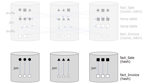
In such a case, you can apply hash distribution strategy for a large table as follows.
The hash distribution will distribute data (not replicate) along with the hash of a distribution column. For instance, if you use hash distribution strategy for fact_Sale table and specify [WWI Invoice ID] as a distribution column, the rows of fact_Sale table will be distributed along with the hash value of [WWI Invoice ID].

DROP TABLE [wwi].[fact_Sale];GOCREATE TABLE [wwi].[fact_Sale]...WITH(   DISTRIBUTION = HASH([WWI Invoice ID]),  CLUSTERED COLUMNSTORE INDEX)DROP TABLE [wwi].[fact_Invoice];GOCREATE TABLE [wwi].[fact_Invoice]...WITH(   DISTRIBUTION = HASH([WWI Invoice ID]),  CLUSTERED COLUMNSTORE INDEX)

The common hash keys have the same data format, even when it’s in a different table.
Thus, if you set [WWI Invoice ID] as a distribution column for both fact_Sale table and fact_Invoice table, the each row for both tables will be distributed in the same database for the same [WWI Invoice ID] value.
Eventually, no shuffle occurs.

However, keep in mind that data type in join columns should exactly be same to get optimal performance. For instance, BIGINT value is differently hashed from INT value, even when it has same values.
In general, all join or comparison operations (such as, WHERE … IN, WHERE … EXISTS, etc) should have same data type between target columns for performance optimization.

Note : Use DBCC PDW_SHOWSPACEUSED for seeing the skewness (each size in distributions, etc) in a table as follows.

DBCC PDW_SHOWSPACEUSED('wwi.fact_Sale');

ROWSRESERVED_SPACE DATA_SPACE INDEX_SPACE UNUSED_SPACE PDW_NODE_ID DISTRIBUTION_ID2412841 17992  17936  0   56   1   12474028 18424  18368  0   56   1   22099684 15744  15688  0   56   1   3...

When you need more detailed information about skewness in the data, use a dynamic management view, sys.dm_pdw_nodes_db_partition_stats. (See here for details.)

SELECT * FROM sys.dm_pdw_nodes_db_partition_stats   WHERE object_id = OBJECT_ID('wwi.fact_Sale');

In the real case, the data shuffle will happen in more complicated situations.
For instance, let’s see the following CTAS (CREATE TABLE AS SELECT) statement with GROUP BY clause.
In this case, if both fact_Sale and fact_Invoice has round-robin distribution strategy, there will also happen much overheads and you will be waited for a long long time…
However, this overhead will be mitigated, when you distribute both fact_Sale table and fact_Invoice table by the hash distribution with a distribution column, [WWI Invoice ID] .

CREATE TABLE [wwi].[fact_Invoice]WITH(   DISTRIBUTION = ROUND_ROBIN,  CLUSTERED COLUMNSTORE INDEX)ASSELECT  [WWI Invoice ID],  SUM([Quantity]) AS [Quantity],  ...FROM [wwi].[fact_Sale]GROUP BY [WWI Invoice ID];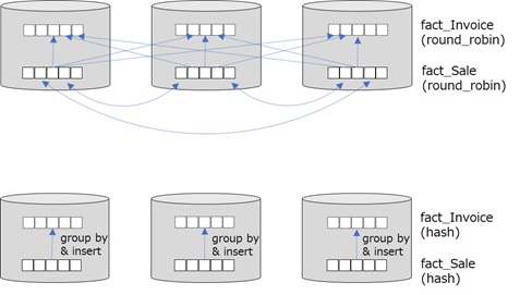

The hash distribution can also be used for optimizing frequent COUNT(DISTINCT) or OVER PARTITION BY .

To get better performance, choose a distribution column which distributes data evenly.

Note : In this post, I described only 2 movement patterns, BroadcastMoveOperation and ShuffleMoveOperation, however, data will be moved by the following patterns in data movement service (DMS).

• ShuffleMoveOperation : Each distributions are distributed by hash algorithm. (i.e, Changing distributions.)
• PartitionMoveOperation : Distributions (in compute node) goes to control node.
• BroadcastMoveOperation : Each distributions are copied into all distributions. (i.e, distributed table to replicate table)
• TrimMoveOperation : Replicated table is distributed by hash algorithm.
• MoveOperation : Data in control node are copied into all distributions (i.e, replicated).

Composite Key

Multi-column distribution (MCD, or multi-column hash) is now generally available in Azure Synapse Analytics dedicated SQL pools. (March 2023)

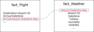
You cannot use multiple columns for a distribution column in hash distribution. When you need multiple columns for distribution key, you should create a new column for hashing as a composite of two or more values.
For instance, suppose, 2 large fact tables, flights and weather, will be joined (combined) with both airport id and date/time. (See the following schema.)

In this case, it’s better to generate a new column (key) as a composite of airport id and datetime, and create tables with hash distribution using this generated new key as a distribution column.

Multiple Strategies For the Same Data

If you needs multiple (different) distribution strategies for the same data, you can use CTAS (CREATE TABLE AS SELECT) to re-create another table with a different distribution column. Or use a materialized view (indexed view), if the definition includes aggregate functions or GROUP BY clause .

A materialized view is a view in database, but it pre-computes, stores, and maintains its data in SQL pool just like a table. There’s no re-computation needed each time when a materialized view is used. You don’t also need to manually maintain a materialized view for the source data change.
However, just like a standard table, a materialized view can also have hash distribution with a distribution column.

CREATE MATERIALIZED VIEW [wwi].[Sale_For_Invoice_View]WITH(  DISTRIBUTION = HASH ([WWI Invoice ID]),  FOR_APPEND)ASSELECT [WWI Invoice ID], MAX([Invoice Date Key]) AS [Invoice Date Key], SUM([Quantity]) AS [Quantity]FROM [wwi].[fact_Sale]GROUP BY [WWI Invoice ID];GOCREATE MATERIALIZED VIEW [wwi].[Sale_For_Customer_View]WITH(  DISTRIBUTION = HASH ([Customer Key]),  FOR_APPEND)ASSELECT [Customer Key], SUM([Quantity]) AS [Quantity]FROM [wwi].[fact_Sale]GROUP BY [Customer Key];GO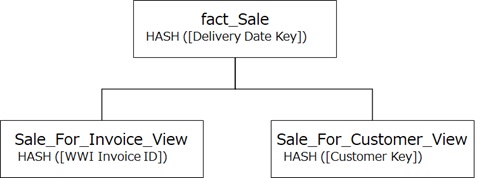

When you run the same query by using SELECT statement (even when not using a materialized view), the optimizer will pick up the corresponding materialized view.

Here I’ve showed you how it works and how to design vertical distributions in Synapse Analytics SQL dedicated pools with several use case.
These ideas for broadcast or shuffle exchange are also used in Apache Spark and the query plan (logical plan and physical plan) in Catalyst optimizer. (You can also see plans with explain() function in Apache Spark SQL or dataframe, and use broadcast() function if you need explicit broadcast joins.) Things written in this post is fundamental and will help you explore the bottlenecks, even in other big-data platforms.

In the next post, I’ll show you the horizontal design in a table using index and partitions.

Useful Reference :

Cheat sheet for Azure Synapse Analytics
https://docs.microsoft.com/en-us/azure/synapse-analytics/sql-data-warehouse/cheat-sheet

Guidance for designing distributed tables in Synapse SQL pool
https://docs.microsoft.com/en-us/azure/synapse-analytics/sql-data-warehouse/sql-data-warehouse-tables-distribute

Design guidance for using replicated tables in Synapse SQL pool
https://docs.microsoft.com/en-us/azure/synapse-analytics/sql-data-warehouse/design-guidance-for-replicated-tables