Welcome to Day2 of my blog series “Synapse Analytics : Designing for Performance”.

1. Optimize for Distributions
2. Choose Right Index and Partition (this post)
3. How Statistics and Cache Works

In this post, I’ll show you how to design data layouts within a table (on single distribution) in Azure Synapse Analytics. This post focuses on indexes and partitions.

Indexing

Designing index for a table is so primitive and important for better performance.
There’s no “one answer for any case”. You should choose right index for a table depending on the size, usage, query patterns, and cardinality.

In order to help you understand pros/cons in each indexes, I’ll show you each pictures illustrating intuitive structures of indexes available in Synapse Analytics.

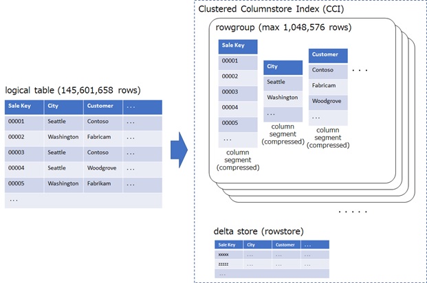
1. Clustered Columnstore Index (CCI)

A clustered columnstore index (CCI) is usually the best choice providing optimal query performance for almost large tables.
By default, Synapse Analytics creates a clustered columnstore index (CCI), when no index options are specified.

CREATE TABLE myTable(  ...)WITH (CLUSTERED COLUMNSTORE INDEX);

Unlike traditional row-oriented index, a columnstore index offers the highest level of data compression by column-based data chunk to provide better performance.
When data is added into CCI table, data is temporarily stored on delta store (which is a rowstore table) in CCI. When the number of rows in delta store reaches to some threshold, then rows are moved into the columnstore.
As a result, each columnstore is divided by some number of rows, called rowgroups. (See below.)

Note : When you use CCI in REPLICATE distribution table, CCI will be generated in each distributions for the first time you run the query. (See my previous post for a replicate table.)

However, when you load large data into CCI table using Polybase (CTAS, Synapse Pipeline, etc) or COPY command, the data will be immediately compressed into columnstore format without inserting into delta store.
For this reason, please avoid loading few data by many separated transactions in Synapse Analytics. (There will be overhead.)

Note : Even when streaming inserts, such as IoT telemetry ingestion, the data will once be saved in temporary location and periodically loaded into Synapse Analytics with bulk in SDK.

This index (CCI) is suitable for large analytical data (ideally, over 100 million rows), such as, transaction data or historical raw data. If a table is small, you shouldn’t use CCI, since the compression ratios will not be efficient.
For optimal compression and performance, 1 million rows are ideal for each rowgroup and you then need at least 1 million rows in each partition.

To see each segments (see above picture) in CCI, run the following query with sys.pdw_nodes_column_store_segments table.
The following example shows row count and disk size in each column segments for a column [Unit Price] in a table [wwi].[fact_Sale].

SELECT  segments.distribution_id AS node,  segments.partition_id,  segments.segment_id AS rowgroup,  segments.row_count,  segments.on_disk_sizeFROM sys.pdw_nodes_column_store_segments AS segmentsJOIN sys.pdw_nodes_partitions AS partitions  ON segments.distribution_id = partitions.distribution_idAND segments.partition_id = partitions.partition_idJOIN sys.pdw_nodes_tables AS nodes_tables  ON partitions.object_id = nodes_tables.object_idAND partitions.pdw_node_id = nodes_tables.pdw_node_idJOIN sys.pdw_table_mappings AS table_mappings  ON nodes_tables.name = table_mappings.physical_nameAND substring(table_mappings.physical_name,40,10) = partitions.distribution_idJOIN sys.columns  ON table_mappings.object_id = columns.object_idAND segments.column_id = columns.column_idWHERE columns.object_id = OBJECT_ID('wwi.fact_Sale')  AND columns.name = 'Unit Price'ORDER BY segments.distribution_id, segments.partition_id, segments.segment_id

node partition_id  rowgroup row_count on_disk_size172057594046840832 01000073   1832172057594046840832 11000043   1896172057594046840832 24127251120272057594046840832 01000125   1752272057594046840832 11000044   1648272057594046840832 24738591472372057594046906368 01000083   1712372057594046906368 11000010   1608...

To see the statistics for each row groups within CCI, use sys.pdw_nodes_column_store_row_groups table instead.

Note : With ordered clustered columnstore index (ordered CCI), the data will be stored by columnar manners (compressed in each column segments), however, the data will be segmented by the sorted order of key column.
For instance, the data will be sorted and segmented by [Delivery Date] column in the following table. If you run query by filtering [Delivery Date] column, it will read only the required segments and eventually this query will be more performant to finish.
(You can also specify multiple columns with ordinals in an ordered CCI.)

CREATE TABLE [wwi].[fact_Sale](  [Sale Key] [bigint] IDENTITY(1,1) NOT NULL,  [Delivery Date] [date] NULL,  [Invoice ID] [int] NOT NULL,  ...)WITH(  DISTRIBUTION = HASH ( [Invoice ID] ),  CLUSTERED COLUMNSTORE INDEX ORDER([Delivery Date]))

The segements will be automatically updated, when you insert, update, or delete data. Hence, loading data into an ordered CCI table can take longer than a non-ordered CCI table.

You can also change a non-ordered CCI table into an ordered CCI table as follows.

CREATE CLUSTERED COLUMNSTORE INDEX [fact_Sale_Index] ON [fact_Sale]ORDER ([Sale Key], [Invoice ID])WITH (DROP_EXISTING = ON)

2. Clustered Rowstore Index (or Clustered Index)

Unlike CCI, this is a row-oriented index (rowstore index). It consists a structure – called B-tree – for a key column, and can then quickly reach to each rows by following B-tree path in filtering data. When you use key column in filtering, the query will be performant, since the entire table is not scanned. (See the following picture.)

There can have only one clustered index per table.

CREATE TABLE myTable(  [Invoice ID] int NOT NULL,  ...)WITH (CLUSTERED INDEX ([Invoice ID]));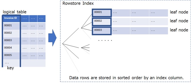

Unlike the following nonclustered index, the data page is stored as a part (in the leaf) of B-tree structure (see above), and additional disk space is not required. Then a clustered index on the sorting column can also avoid the sorting operation.

This index is suitable, when the data is not so large and CCI is not appropriate, such as a dimension table.

Rowstore indexes (including the following nonclustered index and heap table) are ideal for the generic relational database, and please refer SQL Server document for details about anti-patterns, tuning, or access monitoring in rowstore index. (In this post, I don’t go so far about rowstore index.)

3. Nonclustered Index

Like a clustered rowstore index, it also consists a structure of B-tree. However, unlike a clustered rowstore index, the index exists separately from a table. (See the below picture.)
Hence, when the query needs to retrieve non-key data in a row, it happens a “lookup” for row data, even when key is used for filtering.

CREATE TABLE myTable(  ...  City varchar(20),  ...  Customer varchar(20),  ...)WITH ... ;-- Nonclustered Index 1CREATE INDEX cityIndex ON myTable (City);-- Nonclustered Index 2CREATE INDEX customerIndex ON myTable (Customer);

Unlike a clustered index (both columnstore and rowstore), a nonclustered index is a secondary index and can be created on any of other primary indexes (clustered rowstore/columnstore index and heap table).
Mutiple nonclustered indexes can also be created on a single table.
However, too many nonclustered indexes will affect both space and processing time to load.

4. Heap

Use a heap table for a small lookup table or a staging table.

If the table is a heap (and doesn’t have any nonclustered indexes), then the entire table must be read (i.e, a table scan) to find any row. In general, a table scan generates many disk I/O and can be resource intensive. However, if a table is so small, a heap will be efficient for lookup. (See here for the structure of heap.)

CREATE TABLE myTable(  ...)WITH(HEAP);

Loads to heaps are also faster than to other index tables.
Then you can also use heap tables for temporarily landing tables or staging tables.

Note : When you create a materialized view (see my previous post), CCI will be also generated.

Partitioning

You can also use partitions in a table to optimize I/O, but setting partition is optional. (Don’t specify partitions, if it’s not needed.)
When you don’t specify partitions, only one partition on each distribution is used in a table.

Let’s see the example.
Suppose, we create partitions for a table as follows.

CREATE TABLE [wwi].[fact_Sale]WITH(  CLUSTERED COLUMNSTORE INDEX,  DISTRIBUTION = HASH([Invoice ID]),  PARTITION  ([Delivery Date] RANGE RIGHT FOR VALUES('2001-01-01','2002-01-01','2003-01-01')  ))ASSELECT * FROM seed_Sale;

Note : By “RANGE RIGHT FOR VALUES” clause, each boundary value (such as, ‘2001-01-01’, ‘2002-01-01’, and ‘2003-01-01’) belongs to the upper range. When you want these values to belong to the lower range, please use “RANGE LEFT FOR VALUES” instead.

With this DDL command, table data in each distribution will be divided into 4 partitions with the following ranges. If there is 60 distributions, there will be created totally 240 partitions for this table.
Synapse SQL pool supports one partition column (which can be ranged partition) per table.

• Delivery Date : – 2000/12/31
• Delivery Date : 2001/01/01 – 2001/12/31
• Delivery Date : 2002/01/01 – 2002/12/31
• Delivery Date : 2003/01/01 –

Note : In order to see the partition’s definitions in database, please use partition catalog, sys.partition_schemes, sys.partition_functions, and sys.partition_range_values.

Please remind that a distribution column is used to optimize the query using JOIN, GROUP BY, or DISTINCT clauses. (See my previous post.)
On the contrary, a partition column can be used to optimize the query using WHERE clause.
As illustrated in the following picture, if [Invoice ID] is a distribution column and [Delivery Date] is a partition column, only one partition in each parallel distributions will be looked-up by the following query. (Other partitions will be skipped.)

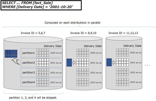
Fig. [Invoice ID] is a distribution column and [Delivery Date] is a partition column

What if you use [Invoice ID] as a partition column and [Delivery Date] as a distribution column (vice versa) in above query ?
In this case, the query will scan all partitions within a single distribution and other distributions are not used. Eventually it will result into degradation of performance.
Do carefully design tables, indexes, and partitions along with query patterns.

Partitioning can also be used for optimization in data management, not only in query.
Suppose, you have a huge historical data. The recent data is often used, but others (old ones) are rarely used and will be archived or removed from database periodically.
These old data could be deleted by using DELETE statement. However, deleting large data row-by-row can take too much time. (Since indexes will be also updated.)
The optimal approach is to drop old partitions and it could take seconds.

If you have a huge historical raw data and it’s always used (referred) by specific years, it might be the time to use partitions on this table.

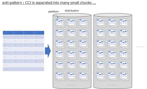
You can use partitions with every indexes, and each indexes will then be separated by each partitions.
Especially, you should take care, when using a clustered columnstore index (CCI). CCI will also be divided into each partitions (see below).

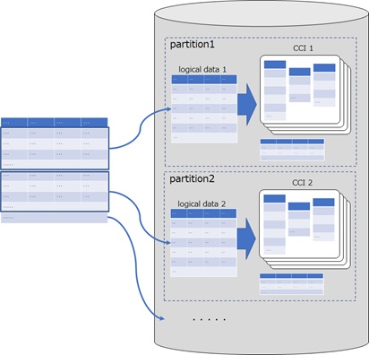
As a result, the rows might be divided into small chunks, and it then might cause the degradation of performance. (As I mentioned above, it’s ideal for CCI to include at least 1 million rows in each partition for optimal performance.)
As I mentioned above, CCI is frequently used in Synapses Analytics. If you just need row segmentation in CCI table, please consider using ordered clustered columnstore index (ordered CCI). (See above note for ordered CCI.)

When you check each number of rows in every partitions, please run the following command.

SELECT  partitions.distribution_id AS node,  partitions.partition_number AS num,  partitions.rowsFROM sys.pdw_nodes_partitions AS partitionsJOIN sys.pdw_nodes_tables AS nodes_tables  ON partitions.object_id = nodes_tables.object_idAND partitions.pdw_node_id = nodes_tables.pdw_node_idJOIN sys.pdw_table_mappings AS table_mappings  ON nodes_tables.name = table_mappings.physical_nameAND substring(table_mappings.physical_name,40,10) = partitions.distribution_idWHERE table_mappings.object_id = OBJECT_ID('wwi.fact_Sale')ORDER BY partitions.distribution_id, partitions.partition_number

node num rows11   160523112   160281713   160228814   160250521   162232322   161857123   161641924   161671531   152745832   152488033   152321934   1524127...

Reference :

Cheat sheet for Azure Synapse Analytics
https://docs.microsoft.com/en-us/azure/synapse-analytics/sql-data-warehouse/cheat-sheet