If you’re a beginner for machine learning, you might think that “complex models can represent a real problem more accurately” or “a lot of training makes models better and better”.
But unfortunately these ideas won’t give you a good result in most cases.

In this post, I’ll describe how these ideas badly affect your model.

Table of Contents

1. Overfitting in Statistical Modeling
2. Overfitting in Neural Networks
3. How to Avoid Overfitting (Apply Regularization)

To give concise samples and examples, I’ll separately discuss in statistical models and neural network models (deep learning). However, as discussed in this post later, you will find that these are closely related each other.

This post will also describe mathematical process in overfitting and underfitting. But I won’t use difficult mathematical representations, and I will explain with a lot of samples and visual understandings to build your intuitions.

To be more precise, several things written in this post will change for other models and approaches. For instance, here I’ll show you an example of parametric regression, but things in this post will differ in non-parametric one. I’ll show you a neural network with softmax (or tanh) activation, but things will differ in other activations.
However, it will help you understand some typical cases.

I hope this post might be a gentle introduction for “what is overfitting” and “how to avoid”.

1. Overfitting in Statistical Modeling

For building your intuition, let me start with primitive statistical regression.

Model Complexity Mismatch

First of all, let me explain about overfitting with a brief example of model complexity mismatching.

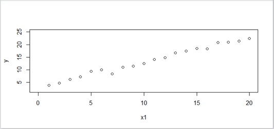
Here I assume that we have the following dataset (training set) :
Now we want to find a mathematical representation to fit this dataset (sample data) with parametric regression.

Figure 1 : Sample data (sampledat)

The following R script is an example for training with simple linear regression (Gaussian regression) model. The following sampledat in this script is the above dataset (a set of and ).

In order to fit precisely in the given data, here I use so flexible linear model with the formula by poly() function. If the result is , then .
The more, the merrier !

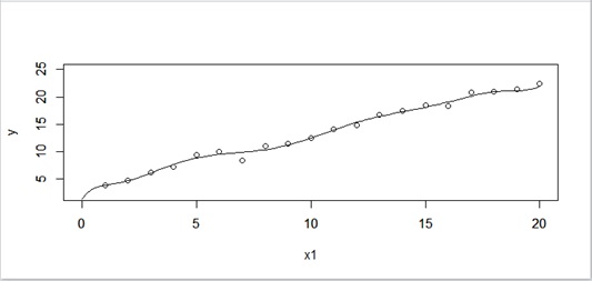
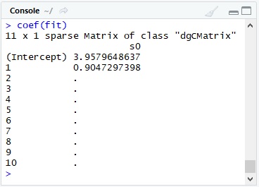
fit <- lm(  y ~ poly(x1, 10, raw = TRUE),  data = sampledat)

However this idea will lead you to a bad result.
First, I’ll show you the result for this regression as follows.

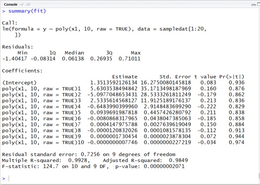
As you can see in above output, I have the following equation (1) to fit for given data.

Now let me plot this equation with the given dataset.
As you can see in Figure 2, it seems that the equation (1) is well fitted to the given data so far …

Figure 2 : Curve of fitted function (10 dimension’s polynomial) – Overfitting

Is that really good result ?

In fact, this given sample data is generated by the following R script.
As you can see below, this dataset is given by with some noise.

n_sample <- 20w0 <- 3w1 <- 1x1 <- c(1:n_sample)epsilon <- rnorm(  n = n_sample,  mean = 0,  sd = 0.7)  # noisey <- w0 + w1 * x1 + epsilonsampledat <- data.frame(  x1 = x1,  y = y)

Now let’s plot our result (equation (1)) for other values of . (See the following Figure 3.)
You will find that this equation fits to only the given data (range in ), but doesn’t fit to the unseen data. This result won’t obviously be the expected one.

Figure 3 : Previous function in bird’s eye view – Overfitting

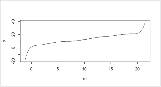
This result (equation (1)) is called overfitting. In overfitting, the model is not generalized for the unseen data.
On contrary, it’s called underfitting when the model is poor and it cannot well represent for data. For instance, when you train the model of 2 dimensional polynomial for dataset generated by 3 dimensional polynomial with noise, the trained model cannot be fitted to the given data.
Of course, overfitting and underfitting can also be seen in a variety of models, not only in regression models – such as, classification, clustering, etc.

In model fitting, there exists an indicator (metrics) called “model bias”, which indicates the average difference between actual data and predicted data. On the other hand, there also exists an indicator called “model variance”, which indicates the model difference in each different training dataset (i.e, model flexibility).
As you saw here, the complex model (such as, 10 dimension polynomials in previous example) will have low bias, but large variance. (When data differs, the model will be largely differ.)
There is a trade-off between “bias” and “variance”, and we then should find an optimal model which has the best balance between model bias and model variance.

Here I showed you a trivial example, but, in practices, it will be difficult to distinguish whether it’s overfitting or not.
Our next concern is :  “How to avoid ?” or “How to detect ?”

Information Criterion in Statistical Models

Later in this post (“3. Avoid overfitting”), I’ll show you several methods for avoiding (or mitigating) the overfitting.
In this section, I’ll briefly introduce some useful indicator (metrics) to find overfitting, which is used in primitive statistical models.

When all parameters are well determined in statistical model, you can use information criterion to find the appropriate number of parameters. (And you could then set the appropriate formula in above lm() function to avoid overfitting.)
There exist several information criterions, such as, Bayesian Information Criterion (BIC) and Akaike Information Criterion (AIC). In this post, I’ll show you AIC examples.

Note : In this post, I use information criterion without any proof.
In both ideas (AIC and BIC), it’s commonly given by , where is the maximum likelihood, is the number of parameters, and is the coefficient depending on each criterion. In AIC, (constant value).
If the dataset is small, it will be difficult to know whether it’s noise or not. In BIC, it includes the number of dataset in , based on the idea of Bayesian statistics.
For Bayesian statistics (how it avoids overfitting), see the below “Note” in section 3 (“3. Avoid overfitting”).

The following represents the criterion for measuring AIC, where is the number of parameters and is the maximum likelihood. (See here for the maximum likelihood.)
This equation tells : the smaller value is better fitting.

Now let’s see the results of AIC for previous example.
The following is the plot for log likelihood () and the value of AIC for each number of parameters. The red line shows the value of likelihood, and blue line shows AIC. (In R script, you can easily get these values with logLik() function and AIC() function.)

Figure 4 : AIC plot (with sampledat)

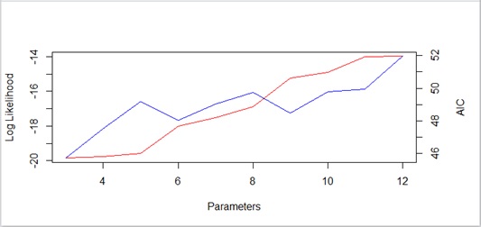
As you can see above, AIC increases more and more, when the number of parameters grows. Thus the appropriate number of estimated parameters will be 3 in this case. That is, the formula will be a good model for fitting for the previous example. (See the following Note.)

Note : The hidden estimated parameters (like the variance for Gaussian, the shape for Gamma, etc) must be counted as estimated parameters in AIC. In this case, we are using Gaussian model, and we must add the variance as one of the estimated and hidden parameters. (See my previous post “Regression in Machine Learning” for details.)
For instance, if the formula (equation) is , then the estimated parameters are , and the variance (i.e, total 3 parameters).

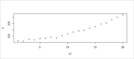
Let’s see another example with the following dataset.
This dataset is generated by 2 dimensional polynomial with some noise.

Figure 5 : Sample data by 2 dimension’s polynomial

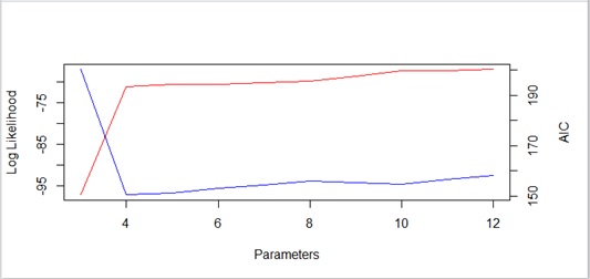
In this case, we’ll get the following AIC.
We can find that the number of parameters should be 4 and the equation (formula) should then be .
Here we can also get the right model by AIC.

Figure 6 : AIC plot (with previous data)

Here I have just used information criterion without any background ideas or any proofs, but the idea of this information criterion is closely related with regularization, discussed in the later section in this post.
Information criterion is supplementarily used for determining the number of parameters in a lot of today’s statistical methods.

Note : The information criterion can be applied under the following conditions :

• parametric approach in statistical model
• all parameters are well determined. (i.e, parameters relatively contribute to the likelihood sensitively, and don’t depend on each other.)

2. Overfitting in Neural Networks

Now let’s proceed our discussion to neural networks (multi-layered perceptron learners, or deep learning), which is inspired by the way computation works in human brain.

Same like previous regression example, the overfitting in neural networks is also due to the complicated (but flexible) and not-generalized models. In this chapter, we’ll see several properties in neural networks with brief examples.

See How Model Complexity Occurs in Neural Networks

Same as previous statistical case (regression example), the complexity (such as, too many layers or neurons) will tend to cause the overfitting also in neural networks.
In neural networks, also it’s not “the more, the merrier”.

A neural network can approximate a wide range of mathematical functions.
For simplicity, here we’ll discuss with feedforward fully-connected neural network to solve a binary classification.
Assume the following network with two numeric inputs () and one binary output (0 or 1), in which the neuron values (0 or 1) of first hidden layer are given by the following activation and other subsequent neurons are given by a logical circuit (e.g, AND, OR, etc…) without weights of previous layer’s values (0 or 1).
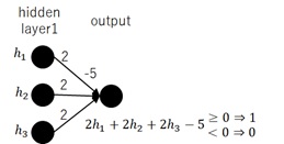
The following Figure 7 is an example of 1 hidden layer and the last layer with logical AND activation. (See the following Note for this unfamiliar network.)

Figure 7 : Example neural network

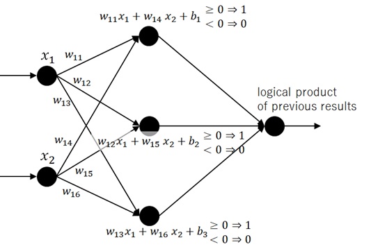
Note : You may think that this example network (with logical operator’s activations and without weights) differs from usual networks used in today’s framework.
It’s known that any logical circuit (“OR”, “XOR”, …) can be represented by using general feedforward networks. This example network will then be equivalent to some parts of general feed-forward networks.

For instance, the following fully-connected network with weights and binary activation is equivalent to the logical product “AND” for binary inputs, 0 or 1.

The multi-layered perceptron networks (MLP) with binary outputs can include any types of complex logical circuits. (The feed-forward neural network represents Borel measurable functions. See studies about function approximators by Hornik et al. (1989), Cybenko (1989), Leshno et al. (1993).)

By using this example (unfamiliar network), I intuitively simplify these binary output’s neural networks.

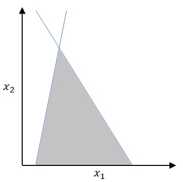
If we have 1 hidden layer (see above network), we’ll have the following illustrated result for numeric inputs () and binary output (0 or 1). In this picture, the gray shaded region means output “1” and others are output “0”.
The result in this picture is the logical combination of multiple linear boundaries by the logical product “AND”.

Figure 8 : Boundary with 1 hidden layer

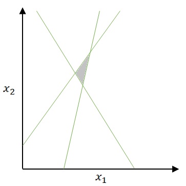
If we have 2 hidden layers, the result will be the combination of above 1 hidden’s results. For instance, in the following picture, I simply combined above 1 hidden’s results with the logical sum “OR”.
Not only protrusion and enclave cases as follows, we could also consider a cavity case or others.

Figure 9 : Boundary with 2 hidden layers

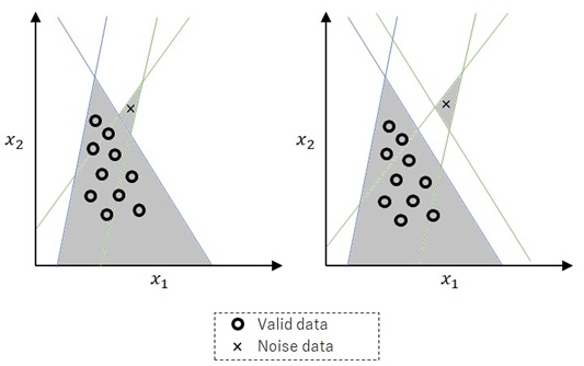
In the following illustration, a circle means a valid data and a cross means a noise data. This noise data is marked as TRUE in experiments, but FALSE in actual.
As you can see in below picture, the neural network with 2 hidden layers might easily cause the overfitting. (In the following illustration, the noise data is also fitted.)

Figure 10 : Overfitting given by the combination of extra layers

By repeating these operations, our simplified neural networks will grow more complicated. If the layer increases, the complexity of model grows rapidly.
As you saw in this section, the number of layers will especially affect to the complexity so much in feed-forward and fully-connected networks.

On contrary, if you apply the simple model with few layers to avoid overfitting, it might increase the risk of underfitting. For instance, when you apply primitive linear (or log-linear) model (where is a weight matrix, is an input vector, and is a bias vector) without hidden layers, it won’t be able to represent even logical “XOR”.
There exists a trade-off between simple models and rich models, and thus we should take care to define complexity (such as, the number of layers or neurons) to represent your problems.

Large Coefficients (Large Parameters)

In this section, you’ll find that the model complexity is easily caused by large coefficients (weights and bias).

Now we consider the activation effects in neural network.
To simplify, let’s discuss with a simple sigmoid activation function. (We will restrict activation to a single target with sigmoid, though the extension to multiple classes (i.e, softmax or tanh activation) is straightforward.)

First of all, the logistic sigmoid function has the following 2 types of parts, linear part and binary part. As you can see in the following curve, the linear part can smoothly fit for targets, but the binary one won’t.

Figure 11 : Binary part and linear part in sigmoid activation

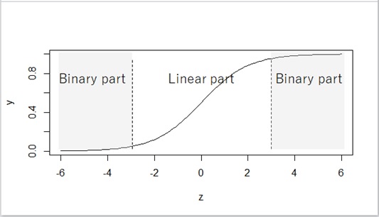
As weights are increased, the effect of binary part will become more stronger than the linear part.

Let’s see this occurrence in the example network.
Here we consider the following fully-connected feedforward neural networks with logistic sigmoid activations. (Each number in the picture is a value of weight and bias.)

Figure 12 : Neural network with small coefficients

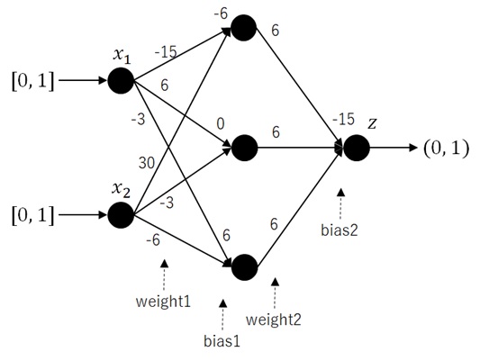
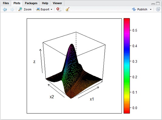
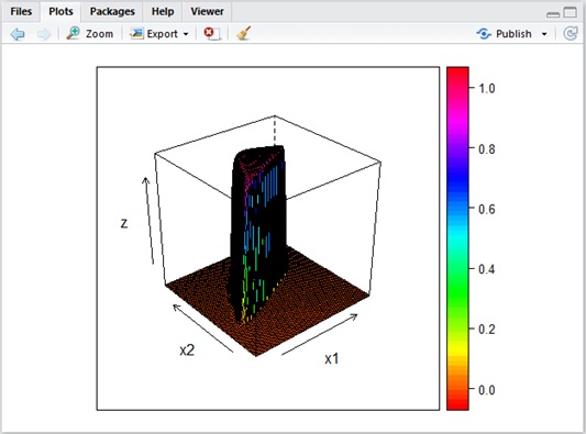
This network (Figure 12) results into the following plots (wire frame). Here is inputs, and z-axis represents an output.
It’s smoothly transitioning by the effects of linear part in sigmoid function.

Figure 13 : Model is smoothly fitted

Now let’s see and compare with the following example.
In the following network (Figure 14), it has the exact same boundary as previous one, but the coefficients (weights and bias) are much larger than Figure 12.

Figure 14 : Neural network with large coefficients

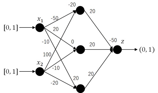
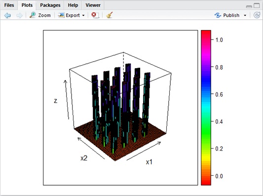
When we plot the inputs () and outputs () as follows, you will find that it loses the smoothness (becomes more sharp), even though it has the same boundary.
In this model, the “binary” part is more characteristic.

Figure 15 : Model is sharp (Compare with Figure 13)

Assume that weights and bias are large and it has too many layers/neurons. The model can easily be complicated or jagged. (See below.)

Figure 16 : Intuition for overfitting by large coefficients (parameters)

As you saw in this example, the large coefficients can easily lead you to the lack of generalization.

Note : The over-fitting can also occur in rectified linear unit activations, such as, ReLU (which doesn’t saturate on both sides), by other reasons, such as, large weight’s update. Also, in this case, the coefficients tend to be large.

In fact, this characteristic (over-fitting with large coefficients) can also be seen in statistical model.
For instance, let’s consider the logistic regression (i.e, logistic sigmoid regression) discussed in my early post. If the dataset “sampledatA” in this example are linearly separable, this gives the boundary , which is equivalent with the boundary . As you can easily see, this will give the solution of maximum likelihood when the magnitude of goes to infinity.

Too Many Training in the Same Dataset

Large coefficients are easily be generated. Assume that you try to train with too many training iterations (i.e, the repeated iterations or epochs) for the same training dataset (inputs).
Each training iteration will increase coefficients slightly (the coefficient’s growth is caused by gradient descent) in order to fit model more precisely to the inputs. By running too many training, this eventually will lead to the complicated model representation.
Of course, less training will give you a poor model (i.e underfitting), but too many training doesn’t also give you a good result. There also exists a trade-off.

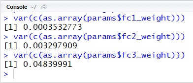
For instance, the following is the simple MXNetR example with feedforward networks for recognizing hand-writing digits (MNIST). At the end of this code, it outputs the variance of each layer’s weights.

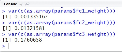
require(mxnet)...# configure networkdata <- mx.symbol.Variable("data")fc1 <- mx.symbol.FullyConnected(data, name="fc1", num_hidden=128)act1 <- mx.symbol.Activation(fc1, name="relu1", act_type="relu")fc2 <- mx.symbol.FullyConnected(act1, name="fc2", num_hidden=64)act2 <- mx.symbol.Activation(fc2, name="relu2", act_type="relu")fc3 <- mx.symbol.FullyConnected(act2, name="fc3", num_hidden=10)softmax <- mx.symbol.SoftmaxOutput(fc3, name="sm")# trainmodel <- mx.model.FeedForward.create(  softmax,  X=traindata.x,  y=traindata.y,  ctx=mx.cpu(),  num.round = 10,  learning.rate=0.07)# dump weights and biasesparams <- model$arg.params# check the variance of weights in each layersvar(c(as.array(params$fc1_weight)))var(c(as.array(params$fc2_weight)))var(c(as.array(params$fc3_weight)))

As you can see the following results, these result coefficients has large value and large variance, when we modify num.round parameter (see above source code) to 100.

epoch = 10

epoch = 100

Note : Learning rate also affects to the weights and accuracy so much. Learning rate must be enough small to constantly decrease the differences in gradient descent, but it must be enough large to make it converge rapidly as possible.
You can experimentally decide this parameter.

I would like to emphasize again that too many training iterations “for the same training dataset” will cause overfitting. If you have large dataset, please don’t hesitate to run the corresponding training iterations. For instance, when you run reinforcement learning, in which the new data will always be supplied, you don’t need to hesitate to keep running the training.
The variation of data (i.e, the data augmentation) will also help you avoid overfitting.

Note : Input’s augmentation, such as – position shift or rotation in images, time shift or levels in voices, etc – is meaningful. Here I don’t go so far, but it’s known to be closely related to tangent propagation regularization technique.
See chapter 5.5.4 – 5.5.5 in “Pattern Recognition and Machine Learning” (Christopher M. Bishop, Microsoft) for details.

3. How to Avoid Overfitting (Apply Regularization)

As you saw above, you can use “information criterion” in primitive statistical models.
But unfortunately, there’s no common criterion for all models including neural network models.

In this section, I’ll list common and typical methods used for mitigating the overfitting today.

Penalty with L1, L2 Regularization

As you saw above, when the model is overfitted, the value (or the number) of parameters tend to be large.
In this section, I’ll show you a method for how to avoid this weight’s increase analytically with penalty terms.
Now let’s see this method in previous linear regression example, .

Before I enter into discussion, I’ll first introduce you a loss function (evaluation function), , where is a weight vector.
A loss function is used for finding a weight vector (i.e, finding a result) which satisfies in the evaluation process. In the previous regression example, the ordinary least square (OLS) will be applied as a loss function. (i.e, where and is the number of training inputs and labels.)
Here I don’t go so far, but see my previous post “Regression in Machine Learning” for details.

In regularization process, we add a penalty term in this evaluation for avoiding weight increase. (See below.)
Even when the loss reduces, the weight might be increased. Therefore the weight is determined by considering the tradeoff between loss and weight’s increase.

Now let’s see the commonly used regularizations, L1 (sparse prior) and L2 (gaussian prior).

With L1 regularization or sparse prior (with which the regression is called Lasso regression), we evaluate and find a weight with a penalty term, , where is a regularization coefficient that controls the relative importance of penalty. ( is determined experimentally.)
Then,

When the weight increases, this total evaluation (total loss) will also increase unless the original loss reduces much more.

With L2 regularization or gaussian prior (with which the regression is called Ridge regression), we evaluate with a penalty term, , in which the penalty term is the square of Euclidean distance instead.
Then,

In this post, I don’t go so far about Bayesian statistics, but L2 regularization is equivalent to applying Bayesian inference to the original regression problems. In the outline of Bayesian inference, we first assume normal distribution (Gaussian distribution) for the prior distribution of weights , and then sum up its posterior distribution after applying likelihood estimation. In this process, a loss function will include a equivalent term with above L2 regularization’s penalty.

Note : Suppose the conditional probability (probability density, when it’s continuous) of target is where is a given input and is a given weight vector, the function, , is often used as a loss function in the likelihood estimation. This loss function by negative logarithm is sometimes called a cross-entropy loss function. (This loss function is used to find to maximize the likelihood . Smaller , larger . See “Regression in Machine Learning” for details about how to maximize the likelihood.)
Assuming that is given by a zero-mean normal distribution (Gaussian distribution), you can find that L2 regularization can be interpreted as a negative logarithm of this distribution.

L2 regularization is mostly used for fitting popular evaluation.
On contrary, L1 regularization will drive the calculated weights to more sparse, i.e, many weights will tend to be exact zero in L1 regularization.

Note : Minimizing L2 loss gives the mean of training samples, while minimizing L1 loss gives the median. A few large outliers will influence the mean of data, while median can be largely unaffected.
This shows the reason why L1 regularization tends to be more sparse.

Now let’s change our previous example (regression with 10 dimension’s polynomial) to avoid overfitting with L2 regularization as follows.
In this example, we set 0.75 as a regularization coefficient, .

library(glmnet)fit <- glmnet(  poly(x1, 10, raw = TRUE),  y,  family = "gaussian",  lambda = 0.75)

Note : When you set , the result will become the same as previous overfitting model.

In this modified example, we obtain . As you can see, the overfitting can be easily avoided with L2 regularization, even when a lot of unnecessary parameters are defined in the formula.

Several statistical modeling naturally involves the same effects with regularizations in its own ideas. For instance, support vector machines (which is often used in classification problems) will prevent overfitting by introducing the idea of margins. (See “Mathematical Introduction for SVM and Kernel Functions” for details.)

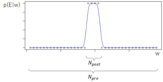
Note : As I mentioned above, Bayesian statistics will also mitigate overfitting in its nature. Here I’ll intuitively show you how Bayesian inference can suppress the overfitting.
Suppose, some model is given and it has only one parameter , and its parameter’s value (value of ) is unknown. Now we consider a marginal likelihood (where is a training set), which is given by :

For simplicity, here we assume the discrete distribution, such as :

• In a prior distribution, the number of possible is , and each has the exact same probability. Then the value of each probability (in prior distribution) is .
• In a posterior distribution, it has maximum probability for all values of , and for others (all values). (See below picture.)

On this assumption, we will obtain :

Then,

If the parameter () finely fits the data in this model (i.e, overfitting), will become large, but will become negatively large (i.e, small), because is always smaller than and will then become close to . (See below.)

The second term works as a model penalty.

Here I assumed only 1 parameter, but if the number of possible parameters increases (i.e, the dimension of increases), the second term will become more negatively larger. Here I don’t go so far, but this result and applying Laplace approximation (Taylor series) will give you a criterion of BIC. (See above description about information criterion, AIC and BIC.)

This method (L1, L2) is also applied to neural network modeling and it’s known as “weight decay” penalty in deep learning.
Same as above, a penalty term for avoiding weight’s increase will be added on optimizer (such as, gradient descent optimizer) in each training iteration of deep learning. For instance, the following code applies L2 regularization in PyTorch optimizer.

# L2 regularization in PyTorchimport torch...sgd = torch.optim.SGD(  model.parameters(),  lr=0.1,  weight_decay=0.9)

There exists an alternative choice called Elastic-Net regularization. The elastic-net regularization combines both L1 and L2 regularization as follows.

where and are penalty terms in L1 and L2 respectively.

This idea of penalty is also applied on pruning algorithm in tree-based model.
Assume that is a tree, is the number of node, and is the loss in each node in tree . The following value (which depends on ) will then be used for the pruning criterion to minimize this value. :

where is a regularization coefficient.

Here I don’t go so far, but tree-based model is also closely related with the model combination idea discussed in the following section. Tree-based model has a separate model (possibly, for both regression and classification) to predict the target label within each region of tree.

Bagging and Dropout (Ensemble Approach)

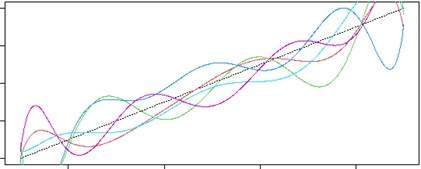
Recall from Figure 2 that when we trained multiple polynomials using this example data, and we can then expect it will be averaged the resulting functions leading to the improved predictions, by the contribution arising from the variance terms tended to be canceled. This method is called Bagging. (The following plotting is the intuitive example for bagging.)

Figure 17 : Ensemble with multiple fitting (called “Bagging”)
– The black dotted line is the average of  trained models.

This ideas of ensemble learning is sometimes referred as Committees.
The above primitive bagging is one of committee examples, but it sometimes cannot be used in practice, because it won’t work well when each models are highly correlated.
Boosting is the improved and often-used committee methods for statistical modeling, in which, multiple models are trained and weighted in sequence by using the previous model to improve performance in the subsequent training. (There also exist parallel (not sequential) approaches to improve in ensemble, such as “Random Forest”.)
I don’t describe how it works in this post, but please refer AdaBoost (adaptive boosting) algorithm for introduction. LightGBM and XGBoost are sophisticated boosting methods and now very popular, both which are based on tree decisions.

This ensemble approach is also applied in neural network modeling.
One of well-used approach (called Dropout) is a method to randomly drop the neurons in each training phase. (See below.)
This method also expects the generalization by model combination and neuron’s co-adaptation.

Figure 18 : Dropout in neural network

In neural networks, it’s experimentally known that the dropout will work well especially with ReLU activations. A lot of frameworks (such as, TensorFlow, Keras, PyTorch, …) natively supports dropout method in functions.
For instance, the below code is the dropout example in PyTorch. (Just use Dropout() or Dropout2d() in the structure as follows.)

# PyTorch model def with Dropoutclass MyTestNet(nn.Module):  def __init__(self):super(MyTestNet, self).__init__()self.layer1 = nn.Sequential(  nn.Conv2d(1, 10, kernel_size=5),  nn.MaxPool2d(kernel_size=2),  nn.ReLU())self.layer2 = nn.Sequential(  nn.Conv2d(10, 20, kernel_size=5),  nn.Dropout2d(),  nn.MaxPool2d(kernel_size=2),  nn.ReLU())self.classifier = nn.Sequential(  nn.Linear(320, 50),  nn.ReLU(),  nn.Dropout(0.5),  nn.Linear(50, 10))self.drop_out = nn.Dropout(0.5)self.fc2 = nn.Linear(50, 10)  def forward(self, x):out = self.layer1(x)out = self.layer2(out)out = out.view(-1, 320)out = self.classifier(out)return out

See here (Wager et al. 2013) for the relation between dropout and L2 regularization.

Early Stopping

The trivial, but practical ways to find out overfitting is to check experimentally. If the accuracy is worse (the loss is more larger) in validation dataset, you will find that it could be overfitting.

Early stopping is a method to evaluate generalization errors in each epochs, and stop learning if the error exceeds some threshold. As you saw above, this is based on the idea of preventing too many training.
A lot of deep learning frameworks also support this method as functions. (See below.)

# Early stopping in PyTorchfrom pytorchtools import EarlyStopping...# initializeearly_stopping = EarlyStopping(  patience=20,  verbose=True)...# check to early stopearly_stopping(loss, model)if early_stopping.early_stop:  break