Get Started with Optimization in Azure Quantum (Simulated Annealing)

By Tsuyoshi Matsuzaki on 2022-07-01• ( 1 Comment )

Important Note : Quantum-inspired optimization solutions are no longer part of the Azure Quantum service after June 30th, 2023. The Microsoft QIO and 1QBit optimization solvers are deprecated and aren’t available. (See here)

In my early posts, I have introduced Q# implementation for several fundamental algorithms in quantum gate’s operations.
However, this kind of general-purpose quantum gate’s operations have difficulties for adoption in real industries today – the most significant one is the error correction problems in scaling.
In quantum adoption, quantum annealing or quantum-inspired computation (i.e, simulating the quantum effects on classical computers) are often applied in today’s industries.

In this post, I’ll introduce you a simple optimization example “Job Shop Scheduling” (a primitive combinatorial problem), which is used in Azure Quantum docs.

Quantum-inspired optimization is a method which emulates quantum tunneling (see here), and uses a concept from quantum physics known as adiabatic theorem. (Shortly, this theorem tells that : as long as transformation happens slowly enough, the system will be expected to adapt in that lowest energy configuration.)

In this post, I’ll apply simulated annealing method in Microsoft QIO (which is one of Azure Quantum provider) to find optimal values in search space.
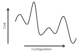
In simulated annealing, a walker ideally moves downhill (toward optimal cost) in search space, but, unlike gradient descent used in generic machine learning, it can also take uphill moves with some non-zero probability. This will then prevent to stuck into sub-optimal local minimum, and it’s then expected to reach to global minimum. (However, I note that it’s not always guaranteed to reach to global minimum.)
Because of this behavior, simulated annealing will be effective in complicated, rugged, but structured landscape in search space.

Note : Unlike quantum annealing, it doesn’t use quantum tunneling effects, but it emulates by downhill and uphill moves (called thermal jumps).

I note that you can also take other methods (rather than simulated annealing) for solving same problems, and the quantum-inspired idea isn’t limited to optimization.
Please see here for other methods, and also check other providers and solvers (such as, 1QBit, Toshiba SQBM+) to run quantum-inspired optimization in Azure Quantum.

What we build … (Job Shop Scheduling)

Job Shop Scheduling example is a famous “Hello World” example in Azure Quantum.
In this example, we will solve a problem to find when to start each operation under some constraints.

First, we have 3 components – operations, jobs, and machines.
To simplify our example, we assume 3 jobs and each job has 2 operations. (It has then total 6 operations.)

Note : In this post, I have simplified example for your very beginning.
See the original example, when each job has different number of operations.

In this example, I assume that the allowed starting time for all operations is 5. I also assume that the processing time in each operation is pre-defined as follows.
For instance, when operation #5 starts at time segment 3, then operation #5 will perform a task during time segment 3 and 4 (because the processing time of operation #5 is 2).

Operation #0 : 2
Operation #1 : 1
Operation #2 : 2
Operation #3 : 2
Operation #4 : 1
Operation #5 : 2

In addition, we have 2 machines, and each machine has operations, [#0, #1, #4, #5] and [#2, #3].

Under these conditions, we have the following 3 constraints.

Precedence Constraint : Operations in a job must take place in order.
Operation Once Constraint : Each operation is started once and only once. Once an operation starts, it must run to completion.
No Overlap Constraint : Machines can only do one thing at a time.

In Job Shop Scheduling example, we should find the optimal starting time (timing) in each operation under all these assumptions.

Formulate a problem (Problem configuration)

Now I define $x_{i,t} \in \{ 0,1 \}$ to be a state at operation $i$ and time $t$ . In this notation, if $x_{i,t} = 1$ , it means that operation $i$ starts at time $t$ . If $x_{i,t} = 0$ , operation $i$ does not start at time $t$ .

First we consider to map $x_{i,t}$ into 1D array representation (linear term).
When the time allowed in the operation is $T$ (here $T=5$ ), all possible states in operation $i$ are $x_{i,0}, x_{i,1}, \ldots, x_{i,T-1}$ . Therefore, we can apply mapping $x_{i,t}$ (i.e, the state pf operation i at time t) into 1D array by $x_{i*T+t}$ . (See below.)

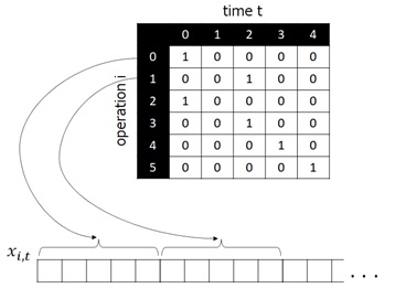
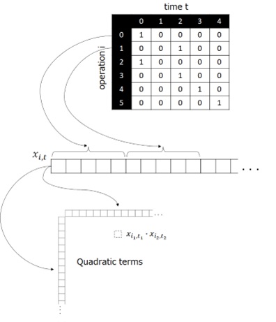
In simulated annealing in this example, we’ll try to represent all conditions by using the following 3 types of terms. (Each term can have 0 or 1 in PUBO model.)

Constant Term : Represent a constant 1. (always 1)
Linear Term : Represent $x_{i,t}$ in this example.
Quadratic Term : Represent $x_{i_1,t_1} \cdot x_{i_2,t_2}$ in this example. (See below.)

Now let’s consider the constraint #1 (Precedence Constraint) with this notation.
When it doesn’t meet this constraint, there exists $i, t, s$ which satisfies $x_{i,t} \cdot x_{i+1,s} = 1$ and $s < t + p_i$ where $p_i$ is the processing time in operation $i$ .
Hence the loss $f(x)$ of this constraint will be written by :

$\displaystyle f(x) = \sum_{\substack{k_{n-1} < i \leq k_n \\ s < t + p_i}} x_{i,t} \cdot x_{i+1,s}$

where $k_n$ is the last operation’s index in job $n$ . (assume $k_{-1} = -1$ )

If all operations meet the constraint #1, $f(x)$ (i.e, the loss of constraint #1) will then be 0. Otherwise, $f(x)$ becomes greater.

For the constraint #2 (Operation Once Constraint), $\sum_t x_{i,t} - 1$ should be zero for any operation $i$ . (Otherwise, the absolute value of this form becomes greater.)
The total loss of constraint #2 will then be :

$\displaystyle g(x) = \sum_i \left( \sum_t x_{i,t} - 1 \right)^2$

Now let me explain with the assumption of $T=2$ for simplification.
When $T=2$ , the loss $g(x)$ in operation $i$ will be :

$\displaystyle \left( \left( \sum_{t=0,1} x_{i,t} \right) - 1 \right)^2$

$\displaystyle = (x_{i,0} + x_{i,1} - 1)^2$

$\displaystyle = (x + y - 1)^2$

$\displaystyle = x^2 + y^2 + 2xy - 2x - 2y + 1$

(Here I have denoted $x_{i,0}, x_{i,1}$ by $x, y$ .)

As you can find, the loss $g(x)$ depends on terms : $x^2$ (quadratic terms), $2xy$ (quadratic terms), $2x$ (linear terms), and $1$ (constant term).
This also holds, when $T$ is other values, such as, $T=5$ .

The loss of constraint #2 will then be rewritten as follows, using terms. :

$\displaystyle g(x) = \sum_{i,t} x_{i,t}^2 + 2 \sum_{\substack{i \\ t \neq s}} x_{i,t} \cdot x_{i,s} - 2 \sum_{i,t} x_{i,t} + \sum_{i} 1$

Finally, let’s consider the constraint #3 (No Overlap Constraint).
I assume that 2 operations $i$ and $k$ are in the same machine and $x_{i,t} = 1$ . In this assumption, $x_{i,t} \cdot x_{k,s}$ should be zero for any $t \leq s < t + p_i$ , when it meets this constraint.
The total loss of constraint #3 will then be written by :

$\displaystyle h(x) = \sum_{\substack{i, k \in I(m) \\ i \neq k}} \left( \sum_{\substack{t \\ t \leq s < t + p_i}} x_{i,t} \cdot x_{k,s} \right)$

where $I(m)$ is the list of all operations in machine $m$ .

Programming Problems (Python)

Now let’s implement this optimization in Azure Quantum.
In optimization on Azure Quantum, we should use Python to represent problems. (Unlike quantum computing, we don’t use Q#.)

Before starting, create an Azure Quantum workspace in Azure Portal.

Afterwards, select Notebooks in the left navigation.

In the notebook window, create a new empty notebook. (For kernel type in notebook, select IPython.)

Note : Here we build from scratch (from empty notebook), but you can start with “Job Shop Scheduling” example in sample gallery.

When you open the notebook, the following code is automatically included.
By using workspace object, you can connect your workload to solvers in Azure Quantum.

from azure.quantum import Workspaceworkspace = Workspace (  subscription_id = "{SUBSCRIPTION-ID}",  resource_group = "{RESOURCE-GROUP-NAME}",  name = "{AZURE-QUANTUM-RESOURCE-NAME}",  location = "{AZURE-QUANTUM-REGION}")

First, in this example, we define the following parameters.

# Set problem parametersn = 3   # Number of jobso = 2   # Number of operations per jobp = [2,1,2,2,1,2]   # Processing time for each operationT = 5   # The allowed time in a job to complete# Six operations in two machinesops_machines_map = [  [0,1,4,5],  [2,3]]

Let’s build the loss of precedence constraint (“Operations in a job must take place in order”).
As you saw above, the loss of this constraint $f(x)$ is processed as follows, by using terms.

$\displaystyle f(x) = \sum_{\substack{k_{n-1} < i \leq k_n \\ s < t + p_i}} x_{i,t} \cdot x_{i+1,s}$

from typing import Listfrom azure.quantum.optimization import Termdef precedence_constraint(n:int, o:int, T:int, p:List[int], w:float):  """  n (int): Total number of jobs  o (int): Number of operations per job  T (int): Time allowed to complete all operations  p (List[int]): List of job processing times for each operation  w (float): relative weight of this constraint  """  terms = []  j = 0  # Loop through all jobs  while(j < n):# Loop through all operations (except the last operation) in this jobfor i in range(j * o, j * o + o - 1):  # Loop through times:  for t in range(0, T):# Loop over times that would violate the constraintfor s in range(0, min(t + p[i], T)):  terms.append(Term(w=w*1.0, indices=[i*T+t, (i+1)*T+s]))j = j + 1  return terms

Next, build the loss of operation once constraint (“Each operation is started once and only once”).
As you saw above, the loss of this constraint $g(x)$ is processed as follows, by using terms.

$\displaystyle g(x) = \sum_{i,t} x_{i,t}^2 + 2 \sum_{\substack{i \\ t \neq s}} x_{i,t} \cdot x_{i,s} - 2 \sum_{i,t} x_{i,t} + \sum_i 1$

def operation_once_constraint(n: int, o: int, T:int, w:float):  """  n (int): Total number of jobs  o (int): Number of operations per job  T (int): Time allowed to complete all operations  w (float): relative weight of this constraint  """  terms = []  #  # Implement penalty : x^2 + y^2 + 2xy - 2x - 2y + 1  #  # Loop through all operations  for i in range(n*o):# Loop through timesfor t in range(T):  # x^2, y^2 terms  terms.append(Term(w=w*1.0, indices=[i*T+t, i*T+t]))  # -2x, -2y terms  terms.append(Term(w=w*(-2.0), indices=[i*T+t]))  # +2xy terms  for s in range(t+1, T):terms.append(Term(w=w*2.0, indices=[i*T+t,i*T+s]))# +1 termsterms.append(Term(w=w*1.0, indices=[]))  return terms

Next, build the loss of no overlap constraint (“Machines can only do one thing at a time”).
As you saw above, the loss of this constraint $h(x)$ is processed as follows, by using terms.

$\displaystyle h(x) = \sum_{\substack{i, k \in I(m) \\ i \neq k}} \left( \sum_{\substack{t \\ t \leq s < t + p_i}} x_{i,t} \cdot x_{k,s} \right)$

def no_overlap_constraint(T:int, p:List[int], w:float, ops_machines_map:List[List[int]]):  """  T (int): Time allowed to complete all operations  p (List[int]): List of job processing times for each operation  w (float): relative weight of this constraint  ops_machines_map (List[List[int]]): Mapping od operations to machines :ops_machines_map = [  [0, 1, 4, 5],  [2, 3]]  """  terms = []  # Loop over each machine  for m in range(len(ops_machines_map)):# Get operations assigned to this machineops = ops_machines_map[m]# Loop over each other operation, i and k, in this machinefor i in range(len(ops)):  for k in range(len(ops)):# Loop over timefor t in range(T):  if ops[i] != ops[k]:for s in range(t, min(t + p[ops[i]], T)):  terms.append(Term(w=w*1.0, indices=[ops[i]*T+t, ops[k]*T+s]))  return terms

To evaluate total loss, we’ll add all terms $f(x)$ , $g(x)$ , and $h(x)$ with the corresponding weights $\alpha$ , $\beta$ , and $\gamma$ as follows.

$\alpha f(x) + \beta g(x) + \gamma h(x)$

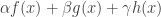
# Assign penalty term weightsalpha = 0.6   # 1.Precedence constraintbeta = 0.2# 2.Operation once constraintgamma = 0.2   # 3.No overlap constraint# Build termsw1 = precedence_constraint(n, o, T, p, alpha)w2 = operation_once_constraint(n, o, T, beta)w3 = no_overlap_constraint(T, p, gamma, ops_machines_map)# Combine termsterms = w1 + w2 + w3

Now we have finished to build penalty (loss) to represent problem constraints.
Afterwards, please optimize your code (such as, reducing terms) for more efficient processing, but I’ll skip this step in this post.

Run Optimization

Now let’s run the optimization.

In simulated annealing method, you can use PUBO (Polynomial Unconstrained Binary Optimization) or Ising model for solvers. In this example, we’re assuming PUBO solver.

Note : In this post, I don’t deep dive into details about solvers (algorithms), but please refer here for details.

from azure.quantum.optimization import Problem, ProblemType, SimulatedAnnealing# Problem type is PUBO in this instanceproblem = Problem(  name="Job shop sample",  problem_type=ProblemType.pubo,  terms=terms)# Provide details of our workspacesolver = SimulatedAnnealing(workspace, timeout=100)# Run job synchronouslyresult = solver.optimize(problem)config = result["configuration"]# Print resultprint(config)

When you run this code, it shows the following output. This output tells which time is the best to start in each operation.

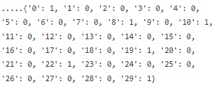
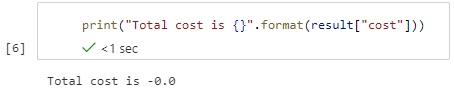
You can also find that the total cost is zero (0.0).

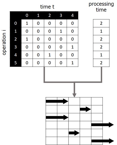
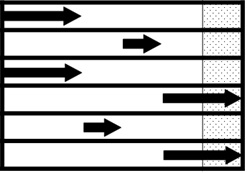
To make things clear, I’ll visualize this result as follows.
Recall that each operation has pre-defined processing time. Each operation will then perform in the following time segment.

Now let’s check whether it meets 3 constraints.

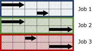
1. Precedence Constraint : “Operations in a job must take place in order.”

In this example, each job has 2 operations in order. (There exist total 3 jobs.)
As you can see below, operations in each job are taking place in order.

2. Operation Once Constraint : “Each operation is started once and only once.”

Obviously, each operation starts task once and only once.

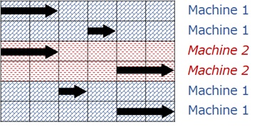
3. No Overlap Constraint : “Machines can only do one thing at a time.”

In this example, there exist 2 machines and each machine has corresponding operations, [0,1,4,5] and [2,3].
As you can see below, there’s no overlap (loss=0) in each machine.

As you saw above, you should formulate problems to fit to the target algorithms (such as, problem configuration, cost function definition, and converting a problem to a model) before programming.
This example is a primitive tutorial, but the formulation in practical problems will not be so easy and need much skills and knowledge for you.

Reference :

Microsoft Learn : Get started with Azure Quantum
https://docs.microsoft.com/en-us/learn/modules/get-started-azure-quantum/

Microsoft Learn : Solve a job shop scheduling optimization problem by using Azure Quantum
https://docs.microsoft.com/en-us/learn/modules/solve-job-shop-optimization-azure-quantum/

GitHub : Scheduling jobs with the Azure Quantum optimization service
https://github.com/microsoft/qio-samples/tree/main/samples/job-shop-scheduling

Categories: Uncategorized

Tagged as: Azure, Quantum

tsmatz

Professional Development, Data Science

Get Started with Optimization in Azure Quantum (Simulated Annealing)

What we build … (Job Shop Scheduling)

Formulate a problem (Problem configuration)

Programming Problems (Python)

Run Optimization

1 reply»

Leave a Reply Cancel reply

Recent Posts

Reinforcement Learning

Imitation Learning

Language Processing

Diffusion Models

Tags

Follow

Get Started with Optimization in Azure Quantum (Simulated Annealing)

What we build … (Job Shop Scheduling)

Formulate a problem (Problem configuration)

Programming Problems (Python)

Run Optimization

Share this:

Related

1 reply»

Leave a Reply Cancel reply

Recent Posts

Reinforcement Learning

Imitation Learning

Language Processing

Diffusion Models

Tags

Follow