Quantum Computing Introduction (Physics & Maths)

By Tsuyoshi Matsuzaki on 2020-03-08• ( 3 Comments )

Many articles describe quantum computing with metaphor, but the goal of this post is to make you understand fundamentals of quantum computing more specifically by referencing the real physics in a very small scale, but without any complicated formula or proofs (with only entry level of physics and mathematics).

The quantum computing uses “Qubit” (=quantum bit) – instead of “Bit” which is used in current popular computing by Neumann architecture. Unlike digital “Bit” in current computers, “Qubit” can never be copied in quantum system. The behavior of this “Qubit” is not easy to understand for humans, and it will then prevent us to understand quantum computing and its properties. The purpose of this post is to make you understand “idea” of this mechanics intuitively, with comprehensive physical examples.

After you have finished reading this post, you will find how it’s represented and used with mathematical notations (such as, braket, tensor, and Bloch sphere representation) and will know the essential meaning of terminologies – such as, superposition, phase, entanglement, and measurement.

Table of contents

Basic Behaviors in Particles (Quantum)
Probability Amplitude
Mathematical Representation
Bloch Sphere
Entanglement
Measurement

Note : “The Feynman Lectures on Physics – Volume III (Quantum Mechanics)” will be a good reading for your entry of quantum mechanics (though it’s a little bit old and not focusing on quantum computing), and my post also then refer to several examples and descriptions from this article.

Basic Behaviors in Particles (Quantum)

First of all, I’ll show how curiously small particles (i.e, quantum) behaves, unlike physical phenomenon we know.

Suppose that we have an electron’s gun. With this device, a lot of electrons will be randomly fired by applying some voltage. (Let’s imagine some kind of apparatus, such as oven.)
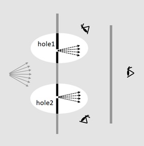
Now we put a wall in front of this gun with 2 slits (2 holes) as below and every triggered electrons will go to this wall. Then only electrons passing through these 2 slits (holes) will eventually reach to the second destination wall.

Figure 1 : Two-slits experiment by electron’s gun

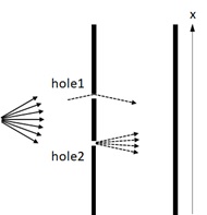
(From “The Feynman Lectures on Physics – Volume III” Chapter 1)

Now we set the detector at destination wall and we plot the total count (the count of electron’s arrival) in each position on x-axis.
Our concern is how this plotting (curve) is going to be ?

I note that the detector at destination wall definitely records each click along with the electron’s arrival. This means that each electron discretely (not continuously) arrives at destination wall. (That is, unlike the wave, you can “count” each electrons.)

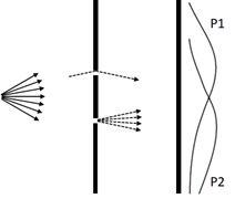
In order to predict this experiment’s result, please imagine that you fire a bunch of bullets with your toy gun. (See below.)
As you can easily see : If hole2 is covered (closed), the total count of bullet’s arrivals will be the following curve P1. If hole1 is covered, the total count will be P2 as well.

Figure 2 : Result with real materials (1)

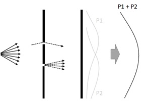
Eventually the expected result (total count) on the destination wall will become P1 + P2 as follows.
When you do this experiment with your toy gun, you will definitely be able to get this exact result.

Figure 3 : Result with real materials (2)

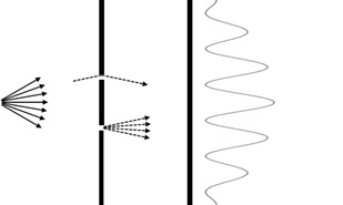
However, in the small scaled quantum world, the result is different from things of our experience !
When we count all electron’s arrivals on the destination wall, the result becomes as follows. Apparently, this is not our expected result.

Figure 4 : Result with particles (atoms)

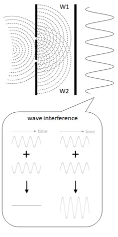
Suppose we do the same experiment with water wave. (See below.)
In this case, each wave through hole1 and hole2 will interfere with each other, and wave’s intensity at destination will then become as following picture.
As you can see, it’s very similar with the result of previous electron’s experiment.

Figure 5 : Two-slits experiment by water

As I mentioned above, each electrons can be detected as each discrete particles, but it also seems to have some sort of wave‘s characteristics (wave-particle duality).
In the things on a very small scale, we can see such an experience that we never had in our real life.

This kind of phenomenon is also observed in quantum’s spin. Now let’s see another experiment.
Let’s say, we consider the following device with magnets, called Stern-Gerlach device. We assume that some particle’s beam (e.g, beam of Ag) is inserted into this device.

Figure 6 : Stern-Gerlach device

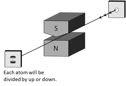
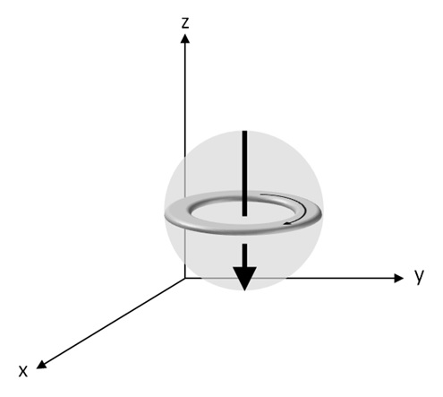
By ununiformed magnetic fields, the current loop in the atom will be pulled into upward or downward, corresponding to anti-clockwise spin or clockwise spin. (See Figure 7 below.)
Eventually, each atom will be divided by upward or downward in the screen (destination), as Figure 6 shows.

Figure 7 : Relation by electron’s spin (current loop) and force in Maxwell’s picture

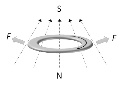
Note : This picture (above example by a single electron’s motion) simplifies the real behavior of electrons to help you understand. It’s known that each electron doesn’t exist in a certain position and it spreads into any space with some uncertainty. This state is called superposition.
In the real experiments, the result of system is caused by various aspects in particles, such as, combination of multiple elements, symmetricity in a molecule, and so on. Depending on the choice of atoms or molecules, the particles might be divided into 3 states – such as, positive (+), zero (0), and negative (-) – in Stern-Gerlach device.

Now we consider the following experiment with the apparatus by combination of 2 Stern-Gerlach devices.
In the first (left) one, we block the downward beam and only pass the upward beam. In the next (right) device, we observe how the beam is divided by upward or downward.

Figure 8 : Experiment with simple combination of Stern-Gerlach’s devices

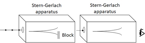
With this experiment, we get the result that all beam becomes upward. (No downward beam is observed.)
This result won’t be strange. (It will be the expected result.)

However, let’s see the following apparatus by 3 devices.
In this experiment, we combine 3 devices such as : In the first one, we block downward beam. (Only upward beam reaches to the next device.) For the next device, we rotate this device around y-axis and block only downward (i.e, crooked direction) beam. With the final device, we observe both upward and downward in the regular direction.

Figure 9 : Experiment with rotated Stern-Gerlach’s filter

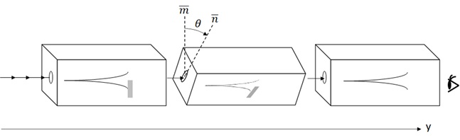
With this experiment, we get the result of both upward and downward ! (i.e, The downward beam can also be appeared again !)
That’s so strange, because we have filtered into only upward beam in the first device.

Probability Amplitude

As you saw in our first example of electron’s gun, these curious results are because of wave-like behaviors.

Note : It’s known that all matter exhibits wave-like behavior and has wavelength $\lambda = \frac{h}{mv}$ (where $m$ is mass, $v$ is velocity, and $h$ is Planck constant). We can comparatively ignore this behavior in almost cases with a large materials, however, we cannot ignore this behavior in quantum-scaled particles.
See Wikipedia “Matter wave (de Broglie wave)” for details.

With a lot of works in physics, this phenomenon is formulated by introducing the idea of probability amplitude, which idea is based on wave’s motion.
The probability amplitude is a complex number which describes behavior in quantum physics.
For now, please think it as an analogy of the following wave’s amplitude $\phi$ . ( $\phi$ will depend on the time $\tau$ .)

Figure 10 : probability amplitude by simple Euler’s formula

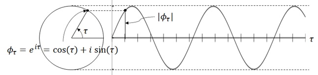
The probability amplitude is not visible and recognizable for humans. As I’ll explain in this section, we can only recognize it as real “probability” $| \phi |^2$ . Figuratively speaking, the probability amplitude is some value in unrecognizable world with “complex number” and we can recognize it as “real number”.

Now let’s remind the previous example of electron’s gun again. (See Figure 1.)
In this example, we can set the probability amplitude as :

$\phi$ : probability amplitude for passing through hole1 and reaching to some position (x) in destination wall
$\chi$ : probability amplitude for passing through hole2 and reaching to some position (x) in destination wall

The summed probability of both paths through hole1 and hole2 is not the sum of probability $\left| \phi \right|^2 + \left| \chi \right|^2$ , but it’s the probability of “the sum of probability amplitude”, i.e, $\left| \phi + \chi \right|^2$ .
As you saw in Figure 5, each $\phi$ and $\chi$ will interfere like the ordinary wave and the result will then become such like Figure 4.

Let’s remind the example of quantum spin again. (See Figure 6.)
In this example, we denote the state of particles which has passed through upward as $m+$ . We also denote the state of particles with downward as $m-$ .
Same like that, we denote the state of particles which has passed through the rotated device (2nd device in Figure 9) as $n+$ . And we also denote the state of opposite side as $n-$ .
Here we can set the probability amplitude as follows. (Please take care of the order !) :

$\left< n+ \middle| m+ \right>$ : the probability amplitude of particles passing through $n+$ after passing through $m+$ . (the probability amplitude of $n+$ with initial state $m+$ )
$\left< n- \middle| m+ \right>$ : the probability amplitude of particles passing through $n-$ after passing through $m+$ . (the probability amplitude of $n-$ with initial state $m+$ )

Note : In the previous example (an example with electron’s gun), you can also denote using bra-ket notation $\left< \ \cdot \ \middle| \ \cdot \ \right>$ .

With this bra-ket notation (called “Dirac notation”), we can describe the probability amplitude in Figure 8 (experiment with simple 2 Stern-Gerlach devices) as follows.

$\left< m+ \middle| m+ \right>$ : the probability amplitude of finding upward particles in Figure 8
$\left< m- \middle| m+ \right>$ : the probability amplitude of finding downward particles in Figure 8

In quantum mechanics, there is a basic principle, such as : $\left< a \middle| a \right> = 1$ . For this reason, you can find :

$\left| \left< m+ \middle| m+ \right> \right|^2 = 1$

and then $\left| \left< m- \middle| m+ \right> \right|^2 = 0$

This means that the real possibility of finding upward particles in Figure 8 is 1, and the real possibility of finding downward particles in Figure 8 is 0.

Next we consider the mixed device of Figure 9 (experiment of 3 Stern-Gerlach devices with rotated one).
First, we can write probability amplitude of particles passing $m+$ on 1st device and $n+$ on 2nd device as $\left< n+ \middle| m+ \right>$ . Then probability amplitude of particles passing $n+$ on 2nd device and $m+$ on 3rd device is $\left< m+ \middle| n+ \right>$ . How can we write the possibility amplitude of “passing $m+$ on 1st device, $n+$ on 2nd device, and $m+$ on 3rd device” ?
In quantum mechanics, this kind of composite possibility amplitude by $\chi$ after $\phi$ is given by the product of complex numbers $\chi \cdot \phi$ . (Please take care for the difference from your familiar “conditional probability”.)

For this principle, each possibility amplitudes for upward and downward in Figure 9 will be :

$\left< m+ \middle| n+ \right> \left< n+ \middle| m+ \right>$ : the probability amplitude of finding upward particles in Figure 9
$\left< m- \middle| n+ \right> \left< n+ \middle| m+ \right>$ : the probability amplitude of finding downward particles in Figure 9

Then the real possibility values of these will be :

$\left| \left< m+ \middle| n+ \right> \right|^2 \left| \left< n+ \middle| m+ \right> \right|^2$ : the probability of finding upward particles in Figure 9
$\left| \left< m- \middle| n+ \right> \right|^2 \left| \left< n+ \middle| m+ \right> \right|^2$ : the probability of finding downward particles in Figure 9

Then the ratio of these values is not depending on which one ( $m+$ or $m-$ ) is selected in the 1st device. (See the following equation.) Even when you have filtered into the upward particles in the first (left) device of Figure 9, the result will then include the downward particles.

$\displaystyle \frac{\left| \left< m+ \middle| n+ \right> \right|^2 \left| \left< n+ \middle| m+ \right> \right|^2}{\left| \left< m- \middle| n+ \right> \right|^2 \left| \left< n+ \middle| m+ \right> \right|^2} = \frac{\left| \left< m+ \middle| n+ \right> \right|^2}{\left| \left< m- \middle| n+ \right> \right|^2}$

When a particle has passed through the 2nd device in Figure 9, the state of this particle is neither $m+$ nor $m-$ . This state is then so-called an intermediate state (for $m+$ and $m-$ ) in quantum physics.
On the other hand, each $m+$ and $m-$ are called base state. As I’ll show you below, all intermediate states are described using the combination of base state.

I note that there exist a lot of set (a lot of pairs, if 2-state system) of base state.
For instance, the pair of $n+$ and $n-$ is also one of base state’s set. The pair of $m+$ and $m-$ is another base state’s set.
The choice of base state is something like a choice of base coordinates in a vector space.

It’s known that there exist the following principles for quantum base state, when $\{ i \} \ (i=0,1, ...)$ is a set of base state. (See chapter 5-5 in “The Feynman Lectures on Physics – Volume III”.) :

$\left< j \middle| i \right> = \delta_{ij}$
i.e, $\left< j \middle| i \right> = 1$ when $i = j$ , and $\left< j \middle| i \right> = 0$ (orthogonal) when $i \neq j$
$\left< \chi \middle| \phi \right> = \sum_{i} \left< \chi \middle| i \right> \left$ for any state $\phi$ and $\chi$

With these principles, when all particles with both $n+$ and $n-$ is passed on the 2nd device in Figure 9, you will find that all observable state in the 3rd device will be m+ as follows.
As you can see, this will be basically the same experiment in Figure 8.

Suppose we have a particle with initial state $\phi$ and this particle goes through some apparatus A (e.g, an apparatus applying some magnetic fields, the combination of multiple Stern-Gerlach devices, and so on). Then the final probability amplitude for $\chi$ is often denoted as $\left< \chi \middle| A \middle| \phi \right>$ using operator A.
For instance, the 2nd rotated device in Figure 9 is also one of these operators and we can denote as A. Using this operator A, we can then denote this experiment as $\left< m+ \middle| A \middle| m+ \right>$ .
In generic gate-model quantum computing, the logic is built by the combination of operators and an operator is sometimes called a gate (circuit).

Through this post, I’ll discuss the quantum computing using an analogy of this quantum spin.

Note : There exist several quantum numbers corresponding to position, momentum, spin, or polarization. Unfortunately there’s no single convenient (complete) formula describing all these aspects.

Mathematical Representation

Up until now, we have considered a complex number value with the notation $\left< \ \cdot \ \middle| \ \cdot \ \right>$ and haven’t divided into bra $\left< \ \cdot \ \right|$ and ket $\left| \ \cdot \ \right>$ .
However, with the idea of mathematical vector analysis, this quantum mechanics is abstracted as Hilbert space using vectors and matrices – i.e, each bra / ket as a vector and an operator as a matrix. (See chapter 8 in “The Feynman Lectures on Physics – Volume III”.)

From now on, we define the following symbols with vectors and matrices. :

$\displaystyle \left| \phi \right> = \begin{pmatrix} \phi_0 \\ \phi_1 \\ \vdots \\ \phi_{n-1} \end{pmatrix}$

$\displaystyle \left< \phi \right| = \left| \phi \right>^{\dagger} = \begin{pmatrix} \phi_0^{*}$

$\displaystyle A = \begin{pmatrix} A_{00}$

For 2-state system, it can be written as :

$\displaystyle \left| \phi \right> = \begin{pmatrix} \phi_0 \\ \phi_1 \end{pmatrix}$

$\displaystyle \left< \phi \right| = \left| \phi \right>^{\dagger} = \begin{pmatrix} \phi_0^{*}$

$\displaystyle A = \begin{pmatrix} A_{00}$

For instance, if $\left| \phi \right> = \begin{pmatrix} a+bi \\ c+di \end{pmatrix}$ is given, $\left< \phi \right|$ is equal to :

$\displaystyle \left< \phi \right| = \begin{pmatrix} a+bi \\ c+di \end{pmatrix}^{\dagger} = \begin{pmatrix} (a+bi)^{*}$

In this algebra, operator A converts some state $\left| \phi \right>$ into $A \left| \phi \right>$ .

Note (Time-Evolution) : When we correctly discuss the actual behavior of particles (which will depend on both time and positions), we should dive into details. In this note, I briefly show you the behavior of time-evolution as follows.
Suppose we have a particle at rest and it has a definite energy $E_0$ . In this situation, it’s known that this particle has the probability amplitude $a e^{-i (\frac{E_0}{\hbar}) \tau}$ depending on time $\tau$ (where $a$ is a position-dependent constant with $\left| a \right| \leq 1$ ). This means that the probability amplitude differs on time $\tau$ .
For instance, when a particle sits in a uniform magnetic field and it has the same direction (moment) of spin for time $\tau$ , the probability amplitude is changed by $a e^{-\frac{i}{\hbar} (-\mu B) \tau}$ (the actual state is multiplied with this value), where $\mu$ is magnetic moment and $B$ is magnetic field.
Furthermore, when we decompose the state as $\left| \phi(\tau) \right> = \sum_{i} \left| i \right> C_i(\tau)$ where $C_i(\tau) = \left$ (see above decomposition principle), it’s known that this system can be written as the following differential equation with some constant $H_{ij} \in \mathbb{C}$ . ( $\hbar$ is the reduced Planck constant, $\hbar = h / 2\pi$ .)
$\displaystyle i \hbar \frac{d C_i(\tau)}{d\tau} = \sum_{j} H_{ij} C_j(\tau)$
This equation can be denoted (rewritten) with the following vector differential equation, called time-dependent Schrodinger equation. ( $H$ is called Hamiltonian operator.)
$\displaystyle i \hbar \frac{d \left| \phi(\tau) \right>}{d\tau} = H \left| \phi(\tau) \right>$
In physics, we can get the time-dependent state (probability amplitude) by solving this Schrodinger equation. (See “The Feynman Lectures on Physics – Volume III”.)
In this post, time-dependent state is not our concerns, and these notations will be omitted to simplify representation. (Hamiltonian will become concerns in other topics, such as, discussing quantum Ising model.)

Suppose the state $\phi$ and $\chi$ are given. As I mentioned in the previous section, we can decompose a probability amplitude using base state as follows :

$\displaystyle \left< \chi \middle| \phi \right>$

$\displaystyle = \sum_{i} \left< \chi \middle| i \right> C_i$

where $C_i = \left$

Hence any $\left| \phi \right>$ can be decomposed using base state as follows. This superposed state (i.e, a liner combination of base state) $\displaystyle \left| \phi \right>$ is called a Qubit state. :

$\displaystyle \left| \phi \right> = \sum_{i} \left| i \right> C_i$

where $C_i \in \mathbb{C}$ and $\sum_{i} \left| C_i \right|^2 = 1$

Note : As I mentioned above : When it’s a stationary state in some energy $E_0$ (such like, in a uniform magnetic field $B$ ), $C_i$ will change depending on time $\tau$ , i.e, $C_i = C_i(\tau) = e^{-i (\frac{E_0}{\hbar}) \tau} C_i(\tau_0)$ where $C_i(\tau_0) \in \mathbb{C}$ is time-independent with some fixed time $\tau_0$ .
Hence, in Qubit’s representation, a state is written by using $C_i = C_i(\tau_0) \in \mathbb{C}$ (time-independent). In Qubit’s representation, $\left| \phi \right>$ is equivalent to $e^{-i \rho} \left| \phi \right>$ for any real number $\rho$ .

Especially in the 2-state system, any qubit states (superpositions) will be written as follows. :

$\displaystyle \alpha \left| 0 \right> + \beta \left| 1 \right>$

where $\alpha, \beta \in \mathbb{C}$ and $\left| \alpha \right|^2 + \left| \beta \right|^2 = 1$

In the quantum computation, the following pair of base state is conventionally used in 2-state system :

$\displaystyle \left| 0 \right> = \begin{pmatrix} 1 \\ 0 \end{pmatrix}$

$\displaystyle \left| 1 \right> = \begin{pmatrix} 0 \\ 1 \end{pmatrix}$

Using this base state, the previous state is written as follows :

$\displaystyle \alpha \left| 0 \right> + \beta \left| 1 \right> = \begin{pmatrix} \alpha \\ \beta \end{pmatrix}$

where $\alpha, \beta \in \mathbb{C}$ and $\left| \alpha \right|^2 + \left| \beta \right|^2 = 1$

Note : $\alpha$ and $\beta$ are simply called as amplitudes of states $\left| 0 \right>$ and $\left| 1 \right>$ , respectively.

Same as above, we can also decompose the formula for any state $\phi$ , $\chi$ , and apparatus (operator) A as follows :

$\displaystyle \left< \chi \middle| A \middle| \phi \right>$

$\displaystyle = \sum_{i,j} \left< \chi \middle| j \right> \left< j \middle| A \middle| i \right> \left$

Each $\left< \chi \middle| j \right>$ and $\left$ is the projection for base state ( $\left| j \right>$ and $\left$ is not depending on $\phi$ and $\chi$ . Hence this equation means that $\left< \chi \middle| A \middle| \phi \right>$ is a linear combination of these projections.
In 2-state’s quantum computation, this A will be the following 2 x 2 matrix :

$\displaystyle A = \begin{pmatrix} \left< 0 \middle| A \middle| 0 \right>$

Now we try to do the simple calculation by quantum states and operations.

Let’s say, now we suppose all particles have the following spin direction and we assume that this state is denoted by $\left| 0 \right>$ . (These particles will go into upward (+z-direction) by previous Stern-Gerlach device.)

Figure 11 : a particle of $\left| 0 \right>$

When we change the state by the following operation called Hadamard (H) gate (which is also physically implemented as some kind of devices or circuits), the converted state is written as follows.
Now we denote this converted state as $\left| + \right>$ .

$\displaystyle H \left| 0 \right> = \begin{pmatrix} \frac{1}{\sqrt{2}}$

When we observe this particle with Stern-Gerlach device of the same direction (+z-direction), we can find that the half of particles go to upward, since $\left| \frac{1}{\sqrt{2}} \right|^2 = \frac{1}{2}$ .

$\displaystyle \left< 0 \middle| + \right> = \begin{pmatrix} 1$

Note : In this experiment, you might think that the half of these particles goes into some state and the other half goes into another state. But, this doesn’t describe particles’ behavior correctly.
You should think that all particles go into some same “uncertain state” (superposition) and we can then observe it as real possibilities and get the half possibility.
Later in “Measurement” section, we’ll go dive into more details.

When you combine 2 apparatus – the particles pass through A in the first device and then pass through B in the next device -, the corresponding operator C (of this combined apparatus) will be : $C = B \cdot A$ (where $B \cdot A$ is the product of each matrix A and B).
With this manner, you can combine a variety of apparatus.

For instance, when you apply Hadamard (H) gate twice, you will find that all state goes back to the original state. (Please try to calculate with matrices.)

Note : Any operators should preserve the state’s norm. Then any operators converting some state to another state should be written as unitary matrix (i.e, a matrix $U$ such as $U U^{\dagger} = I$ ).
See Wikipedia “Quantum logic gate” for other famous unitary operators.
Note : This quantum mechanics explains barrier penetration (also known as quantum tunneling), in which the particle transmits into the second piece of material in some possibilities and uncertainty, even when it’s a large barrier. (Not all particles are reflected by the material.)
We can also explain a variety of other physical phenomena which are never described by classic physical mechanics (such like, half-life of a radioactive element, so on and so forth).
Please read chapter 7-3 in “Feynman Lecture on Physics Volume III”, if you’re interested in these physical behaviors.

Bloch Sphere (Geometric Representation)

Next we consider the geometric representation of qubits.
As you know, a complex number is often represented in 2 dimensional space in mathematics. However, as you’ll find in this section, the geometric representation in 3 dimensional sphere will be so convenient for understanding qubit’s states and operations. (As I have mentioned above, qubit has unit norm and it will then be mapped to sphere.)

Now let’s remind Stern-Gerlach apparatus in Figure 9 again. (See below.)
When we denote the states in 1st and 3rd device as $\left| m\pm \right>$ and the rotated states (states in 2nd device) as $\left| n\pm \right>$ , the probabilities (not probability amplitudes) $P\pm$ of $\left| m+ \right>$ direction for initial states $\left| n\pm \right>$ are experimentally known to be :

$\displaystyle P+ = \frac{1}{2} (1 + \overline{m} \cdot \overline{n})$

$\displaystyle P- = \frac{1}{2} (1 - \overline{m} \cdot \overline{n})$

where $\overline{m} \cdot \overline{n}$ is dot product (inner product), i.e, $\overline{m} \cdot \overline{n} = cos \theta$

Figure 9 (Again)

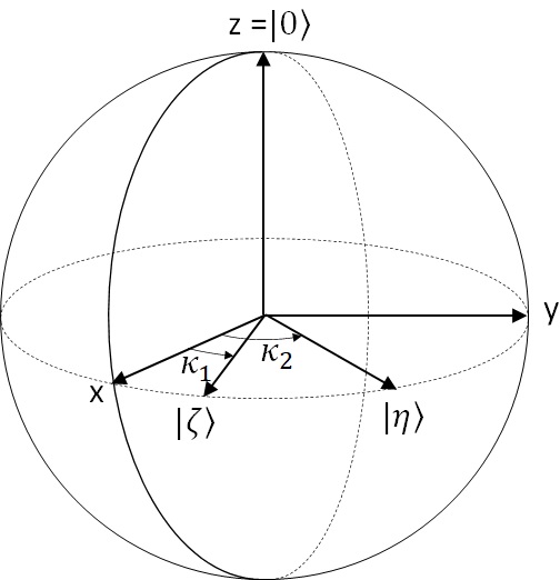
In geometric representation on sphere, now we plot $\left| 0 \right>$ on z-axis, and we set each x and y axis for orthogonal axis (with anti-clockwise order) as follows.
First we assume that we represent the state $\left| \phi \right> = \left| n+ \right>$ in the following sphere, where $\theta$ is the angle between $\overline{0}$ and $\overline{\phi}$ in Stern-Gerlach devices.

Figure 12 : Base sphere

Our concern in this section is how the following $\alpha$ and $\beta$ is represented in above geometric sphere ?

$\displaystyle \left| \phi \right> = \alpha \left| 0 \right> + \beta \left| 1 \right>$

When it’s given the initial state $\left| \phi \right>$ , then the probability (not probability amplitude) of state $\left| 0 \right>$ is $\left| \alpha \right|^2$ . As I mentioned above, this is equal to either $P+$ or $P-$ .
Here we assume that this is equal to $P+$ , then :

$\displaystyle \left| \alpha \right|^2$

$\displaystyle = \frac{1}{2} (1 + \overline{0} \cdot \overline{\phi})$

$\displaystyle = \frac{1}{2} (1 + cos \theta)$

$\displaystyle = cos\left(\frac{\theta}{2}\right)^2$

Then we will get $\left| \alpha \right| = cos(\frac{\theta}{2})$ .
Using the same calculation, we will also get $\left| \beta \right| = sin(\frac{\theta}{2})$
(Same like this, if we have chosen $P-$ , then we will get $\left| \alpha \right| = sin(\frac{\theta}{2})$ and $\left| \beta \right| = cos(\frac{\theta}{2})$ .)
Hence, we will be able to write $\left| \phi \right>$ as follows. (See the following note.) :

$\displaystyle \left| \phi \right>$

$\displaystyle = cos\left(\frac{\theta}{2}\right) e^{i\mu}\left| 0 \right> + sin\left(\frac{\theta}{2}\right) e^{i\nu} \left| 1 \right>$

$\displaystyle = cos\left(\frac{\theta}{2}\right) \left| 0 \right> + sin\left(\frac{\theta}{2}\right) e^{i\kappa} \left| 1 \right>$

where $0 \leq \theta \leq \pi, 0 \leq \kappa < 2\pi$

Note : Here we used the qubit’s property, such as : $\left| \phi \right>$ and $e^{-i\mu} \left| \phi \right>$ is equivalent for any real number $\mu$ . (See above note.)

Next we consider the following 2 states, $\left| \zeta \right>$ and $\left| \eta \right>$ , on x-y plane.

Figure 13 : 2 states on x-y plane (1)

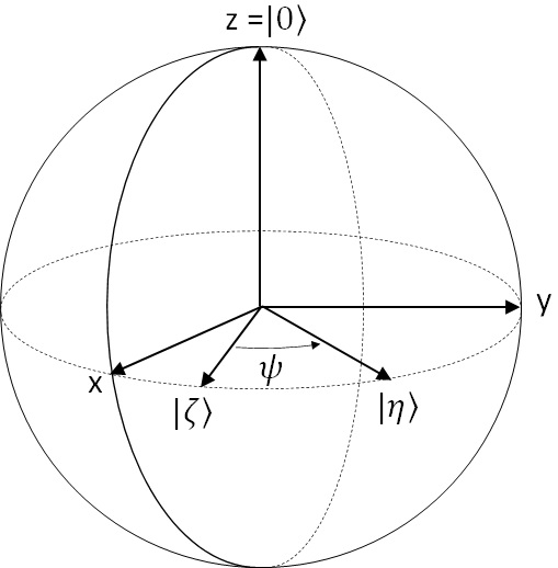
On this plain (x-y plain), $\theta = \frac{\pi}{2}$ , then we can write $\left| \zeta \right>$ and $\left| \eta \right>$ as follows.

$\displaystyle \left| \zeta \right> = \frac{1}{\sqrt{2}} \left| 0 \right> + \frac{1}{\sqrt{2}} e^{i\kappa_1} \left| 1 \right>$

$\displaystyle \left| \eta \right> = \frac{1}{\sqrt{2}} \left| 0 \right> + \frac{1}{\sqrt{2}} e^{i\kappa_2} \left| 1 \right>$

When it’s given the initial state $\left| \zeta \right>$ , then the probability (not probability amplitude) of the state $\left| \eta \right>$ is :

$\displaystyle \left| \left< \eta \middle| \zeta \right> \right|^2$

$\displaystyle = \left| \left(\frac{1}{\sqrt{2}} \left< 0 \right| + \frac{1}{\sqrt{2}} e^{-i\kappa_2} \left< 1 \right|\right) \left(\frac{1}{\sqrt{2}} \left| 0 \right> + \frac{1}{\sqrt{2}} e^{i\kappa_1} \left| 1 \right>\right) \right|^2$

$\displaystyle = \left| \frac{1}{2} + \frac{1}{2} e^{i(\kappa_1 - \kappa_2)} \right|^2$

$\displaystyle = \frac{1}{2} + \frac{1}{2} cos(\kappa_1 - \kappa_2)$

This should be equal to $P+ = \frac{1}{2} (1 + \overline{\eta} \cdot \overline{\zeta}) = \frac{1}{2} (1 + cos\psi)$ or $P- = \frac{1}{2} (1 - \overline{\eta} \cdot \overline{\zeta}) = \frac{1}{2} (1 - cos\psi)$ .
When we assume it’s equal to $P+$ , then $cos(\kappa_1 - \kappa_2) = cos\psi$ and we get $\kappa_1 - \kappa_2 = \pm{\psi}$ .
This implies that the relation of $\kappa_1$ and $\kappa_2$ is like the following picture.

Figure 14 : 2 states on x-y plane (2)

Here I don’t go so far, but this property holds even when it’s not on x-y plane.

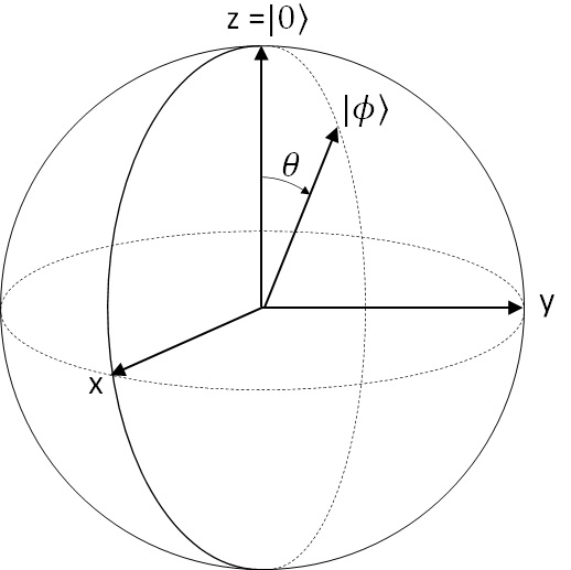
To summarize, any state $\left| \phi \right>$ is uniquely written as :

$\displaystyle cos\left(\frac{\theta}{2}\right) \left| 0 \right> + sin\left(\frac{\theta}{2}\right) e^{i\kappa} \left| 1 \right>$

using the following $\theta$ and $\kappa$ (where $0 \leq \theta \leq \pi, 0 \leq \kappa < 2\pi$ ).

Figure 15 : Bloch Sphere representation

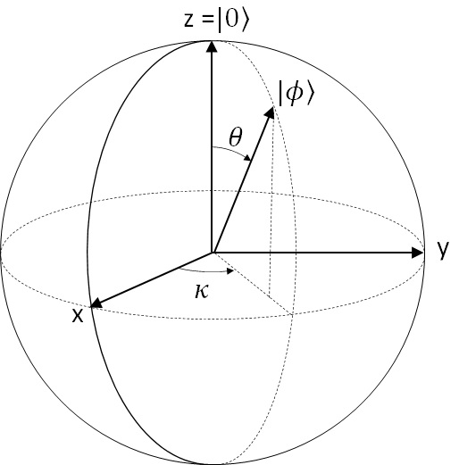
Note : Strictly speaking, only the dipole ( $\left| 0 \right>$ and $\left| 1 \right>$ ) can be written using arbitrary $\kappa$ (not “uniquely written”) in above formula.

This geometric sphere, which describes the qubit’s state, is called Bloch Sphere and it’s useful to consider things, such as the relation of each states, the transformation and combination of quantum logic gates (operations), so on and so forth.
As you can see in this formula, $\theta$ can be observed as probability of bit, but $\kappa$ cannot be observed by humans.

Note : This $\kappa$ is called quantum phase. (As you saw above, $\kappa = | \kappa_1 - \kappa_2 |$ , and it’s then also known as relative phase.)

For instance, when you set $\left| \phi \right> = cos(\frac{\theta}{2}) \left| 0 \right> + sin(\frac{\theta}{2}) e^{i\kappa} \left| 1 \right>$ as one side of a base state’s pair, you can soon get another side of a pair as :

$\displaystyle cos\left(\frac{\pi - \theta}{2}\right) \left| 0 \right> + sin\left(\frac{\pi - \theta}{2}\right) e^{i(\pi + \kappa)} \left| 1 \right>$

$\displaystyle = sin\left(\frac{\theta}{2}\right) \left| 0 \right> - cos\left(\frac{\theta}{2}\right) e^{i\kappa} \left| 1 \right>$

The following well-known Pauli-X ( $\sigma_x$ ), Pauli-Y ( $\sigma_y$ ), and Pauli-Z ( $\sigma_z$ ) gates are operations to rotate $\pi$ radians around corresponding x, y, and z axis in Bloch sphere. (See Wikipedia “Quantum logic gate” for more other logic gates.)
Any single-qubit operation can be written by a linear combination of these 3 gates, since any 2 x 2 matrix can be represented by a linear combination of these matrix.

$\displaystyle \sigma_x = \begin{pmatrix} 0$

$\displaystyle \sigma_y = \begin{pmatrix} 0$

$\displaystyle \sigma_z = \begin{pmatrix} 1$

Note : Pauli-X gate will change the state $\left| 0 \right>$ to $\left| 1 \right>$ , and vice versa. It’s then sometimes called NOT gate.

You will easily be able to find the following equation.

$\displaystyle \sigma_x \sigma_y = i \sigma_z$

$\displaystyle \sigma_y \sigma_z = i \sigma_x$

$\displaystyle \sigma_z \sigma_x = i \sigma_y$

In general, it’s known that the rotation of $\theta$ radians around each axis is written as follows.
You notice that it’s equivalent to the previous $\sigma_x$ , $\sigma_y$ and $\sigma_z$ , if $\theta = \pi$ .

$\displaystyle R_x(\theta) = \begin{pmatrix} cos\frac{\theta}{2}$

$\displaystyle R_y(\theta) = \begin{pmatrix} cos\frac{\theta}{2}$

$\displaystyle R_z(\theta) = \begin{pmatrix} e^{\frac{-i\theta}{2}}$

Note : Here I have also used the qubit’s property, such as :
$\left| \phi \right>$ and $e^{-i\mu} \left| \phi \right>$ is equivalent for any real number $\mu$ . (See above note.)

For instance, previous Hadamard (H) gate is written as the combination of $\pi$ radians rotation around z-axis followed by $\frac{\pi}{2}$ radians rotation around y-axis :

$\displaystyle R_y(\frac{\pi}{2}) \cdot R_z(\pi)$

$\displaystyle = \begin{pmatrix} cos\frac{\pi}{4}$

$\displaystyle = e^{i\frac{\pi}{2}} \cdot H$

As you can find, the rotation of $\left| 0 \right>$ around z-axis is always $\left| 0 \right>$ itself for any $\theta$ radians.

$R_z(\theta) \left| 0 \right>$

$\displaystyle =\begin{pmatrix} e^{\frac{-i\theta}{2}}$

$\displaystyle = e^{\frac{-i\theta}{2}} \left| 0 \right>$

See chapter 10-7 and chapter 11 in “The Feynman Lectures on Physics – Volume III” for details.

Entanglement

After we’ve learned what’s qubit and how to represent the state, now we focus on the important quantum properties – entanglement and measurement.

Suppose there exist 2 species of particles, in which both are also in 2-state system.
In this situation, there exist 4 states by the combination (up-up, up-down, down-up, and down-down) as a set of base state.
This will be equivalent to the following tensor product of each states and denoted by $\left| \phi \chi \right>$ (where each $\phi$ and $\chi$ are 2-state systems).

$\displaystyle \left| \phi \chi \right>$

$\displaystyle = \left| \phi \right> \left| \chi \right>$

$\displaystyle = \left| \phi \right> \otimes \left| \chi \right>$

$\displaystyle = \begin{pmatrix} \phi_0 \\ \phi_1 \end{pmatrix} \otimes \begin{pmatrix} \chi_0 \\ \chi_1 \end{pmatrix}$

$\displaystyle = \begin{pmatrix} \phi_0 \chi_0 \\ \phi_0 \chi_1 \\ \phi_1 \chi_0 \\ \phi_1 \chi_1 \end{pmatrix}$

For instance, when we consider 3 respective different states $\left| \phi \chi \psi \right>$ of particles in 2-state system, we should consider the superposition of 2 x 2 x 2 = 8 state system as follows.

$\displaystyle \left| \phi \chi \psi \right>$

$\displaystyle = \left| \phi \right> \otimes \left| \chi \right> \otimes \left| \psi \right>$

$\displaystyle = \begin{pmatrix} \phi_0 \chi_0 \psi_0 \\ \phi_0 \chi_0 \psi_1 \\ \phi_0 \chi_1 \psi_0 \\ \phi_0 \chi_1 \psi_1 \\ \phi_1 \chi_0 \psi_0 \\ \phi_1 \chi_0 \psi_1 \\ \phi_1 \chi_1 \psi_0 \\ \phi_1 \chi_1 \psi_1 \end{pmatrix}$

When you apply some operator (gate) A and B to respectively $\left| \phi \right>$ and $\left| \chi \right>$ , it’s equivalent to applying $A \otimes B$ to $\left| \phi \chi \right>$ . (See below for this reason.)
It’s a beauty of mathematics.

$(A \otimes B) \left| \phi \chi \right> = (A\left| \phi \right>) \otimes (B\left| \chi \right>)$

These states are often called separable.
For instance, the following $\left| \phi \right>$ is also a pair of separable states.

$\displaystyle \left| \phi \right> = \frac{1}{\sqrt{2}} \left| 00 \right> + \frac{1}{\sqrt{2}} \left| 01 \right> = \left| 0 \right> \otimes (\frac{1}{\sqrt{2}} \left| 0 \right> + \frac{1}{\sqrt{2}} \left| 1 \right>)$

On the other hand, let’s consider the following famous state, called Bell state.

$\displaystyle \left| \chi \right> = \frac{1}{\sqrt{2}} \left| 00 \right> + \frac{1}{\sqrt{2}} \left| 11 \right>$

Unlike above separable state, this is very strange state, because :
Suppose Alice measures the first qubit and Bob measures the second qubit. When Alice measures the first qubit, she will have a 50% chance of measuring $\left| 0 \right>$ and a 50% chance of measuring $\left| 1 \right>$ . On Bob’s side, he will also have a 50% chance of $\left| 0 \right>$ and a 50% chance of $\left| 1 \right>$ . Whereas, if Alice measures the first qubit and get $\left| 0 \right>$ , Bob should measure the second qubit as $\left| 0 \right>$ with a 100% chance (since $\left| 01 \right|^2 = 0$ ), even when the particles are separated by a large distance and they don’t know each other.

Note : Please refer well-known EPR paradox.

Unlike above state, this state can never be algebraically separated by tensor product.
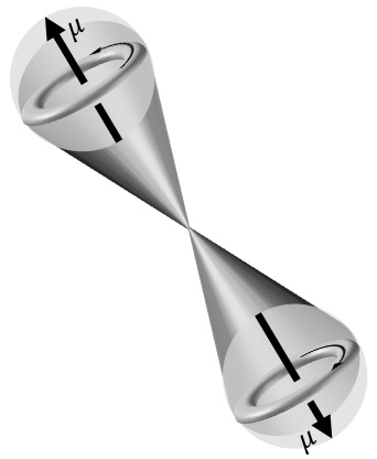
These states (non-separable states) are called entangled state.

Here I don’t go so far, but this strange state actually happens in real particles.
For instance, suppose a pair of electrons are generated together. Then one will have clockwise spin and the other will have anti-clockwise. Even when these are separated by a large distance, this pair will continue to maintain zero total spin.
These 2 states of particles will keep consistent with above quantum rules.

Figure 16 : Entangled State

Entanglement is a very important aspect for quantum computing.

For instance, if you apply some operation to the first qubit in Bell state, the second qubit will also be converted into the same state. (Please calculate with matrices $A \otimes I$ , where $I$ is an identity matrix.)
If there’s n qubits, there exist $2^n$ base state and these are simultaneously converted by entangled state.

Now let’s look at the following practical example, which shows how to use the entanglement in computing.
Suppose some 3-bits parity p = 5 = 101 (2) is given, then we have corresponding 3 qubits as follows. :

$\left| x_i \right> = \begin{pmatrix} \frac{1}{\sqrt{2}} \\ \frac{1}{\sqrt{2}} \end{pmatrix} \ \ (i = 0, 1, 2)$

Next we prepare the following ancilla qubit $\left| x_3 \right>$ .

$\left| x_3 \right> = \begin{pmatrix} \frac{1}{\sqrt{2}} \\ -\frac{1}{\sqrt{2}} \end{pmatrix}$

Now we get the following state. (We denote this state as $\left| \phi \right>$ .) :

$\displaystyle \left| x_0 x_1 x_2 x_3 \right>$

$\displaystyle = \frac{1}{4} \left| 0000 \right> - \frac{1}{4} \left| 0001 \right> + \frac{1}{4} \left| 0010 \right> - \frac{1}{4} \left| 0011 \right> + \frac{1}{4} \left| 0100 \right> - \frac{1}{4} \left| 0101 \right> + \frac{1}{4} \left| 0110 \right> - \frac{1}{4} \left| 0111 \right> + \frac{1}{4} \left| 1000 \right> - \frac{1}{4} \left| 1001 \right> + \frac{1}{4} \left| 1010 \right> - \frac{1}{4} \left| 1011 \right> + \frac{1}{4} \left| 1100 \right> - \frac{1}{4} \left| 1101 \right> + \frac{1}{4} \left| 1110 \right> - \frac{1}{4} \left| 1111 \right>$

$\displaystyle = \left| \phi \right>$

In quantum computing, we can entangle or disentangle 2 states with the following Controlled-NOT operation (CNOT). (It’s written as a non-separable 2-qubit operation.)

$\displaystyle CNOT = \begin{pmatrix} 1$

This CNOT replaces the second qubit, only when the first qubit is $\left| 1 \right>$ . (If the first qubit is $\left| 0 \right>$ , we do nothing for the second qubit.)
Then CNOT converts base states as follows. (Please remind that any states can be written by a linear combination of these base states.)

$\displaystyle CNOT \left| 00 \right> = \left| 00 \right>$

$\displaystyle CNOT \left| 01 \right> = \left| 01 \right>$

$\displaystyle CNOT \left| 10 \right> = \left| 11 \right>$

$\displaystyle CNOT \left| 11 \right> = \left| 10 \right>$

Now we check each i-th bit (i=0,1,2) in parity p, then we apply CNOT for a pair of $\left| x_i \right> \ (i=0,1,2)$ and $\left| x_3 \right>$ , only when i-th bit is 1. (When i-th bit is 0, we do nothing.) We denote this CNOT operation using suffix, as $CNOT_{i3}$ .

In our case, we apply $CNOT_{03}$ and $CNOT_{23}$ , because our parity p = 101 (2).
First, we apply $CNOT_{03}$ . As I mentioned above, this operator replaces the 4th qubit, only when the 1st qubit is $\left| 1 \right>$ .
Hence,

$\displaystyle CNOT_{03} \left| \phi \right>$

$\displaystyle = \frac{1}{4} \left| 0000 \right> - \frac{1}{4} \left| 0001 \right> + \frac{1}{4} \left| 0010 \right> - \frac{1}{4} \left| 0011 \right> + \frac{1}{4} \left| 0100 \right> - \frac{1}{4} \left| 0101 \right> + \frac{1}{4} \left| 0110 \right> - \frac{1}{4} \left| 0111 \right> - \frac{1}{4} \left| 1001 \right> + \frac{1}{4} \left| 1000 \right> - \frac{1}{4} \left| 1011 \right> + \frac{1}{4} \left| 1010 \right> - \frac{1}{4} \left| 1101 \right> + \frac{1}{4} \left| 1100 \right> - \frac{1}{4} \left| 1111 \right> + \frac{1}{4} \left| 1110 \right>$

$= \left| \chi \right> \displaystyle$

Same like this, we next apply $CNOT_{23}$ , then we will get :

$CNOT_{23} \left| \chi \right> \displaystyle$

$\displaystyle = \frac{1}{4} \left| 0000 \right> - \frac{1}{4} \left| 0001 \right> - \frac{1}{4} \left| 0010 \right> + \frac{1}{4} \left| 0011 \right> + \frac{1}{4} \left| 0100 \right> - \frac{1}{4} \left| 0101 \right> - \frac{1}{4} \left| 0110 \right> + \frac{1}{4} \left| 0111 \right> - \frac{1}{4} \left| 1001 \right> + \frac{1}{4} \left| 1000 \right> + \frac{1}{4} \left| 1011 \right> - \frac{1}{4} \left| 1010 \right> - \frac{1}{4} \left| 1101 \right> + \frac{1}{4} \left| 1100 \right> + \frac{1}{4} \left| 1111 \right> - \frac{1}{4} \left| 1110 \right>$

$= \left| \psi \right>$

Finally, we apply the previous Hadamard operator $\begin{pmatrix} \frac{1}{\sqrt{2}}$ for only first 3 qubits ( $\left| x_i \right>$ for i=0,1,2).

$\displaystyle (H \otimes H \otimes H \otimes I) \left| \psi \right>$

$\displaystyle = \frac{1}{\sqrt{2}} \left| 1010 \right> - \frac{1}{\sqrt{2}} \left| 1011 \right>$

Now you got 1010 ( $x_0=1,x_1=0,x_2=1,x_3=0$ ) with a 50% chance and 1011 ( $x_0=1,x_1=0,x_2=1,x_3=1)$ with a 50% chance.
As you can find, the first 3 qubits ( $x_0,x_1,x_2$ ) is always 101 and it’s the same value as our parity p = 101 (2).

Here I don’t go so far, but it’s known that this algorithm holds for any n (> 0) qubits and any parity p. (It’s known as Bernstein-Vazirani algorithm. See here for details.)

As you saw in this example, each qubits are converted maintaining each relations and goes into some totally uniformed state with entanglement effects. As a result, we can observe the consistent results.
Quantum method can form exponentially large space using a uniform state description and transformation, and the entanglement is then used in almost all today’s algorithms.

Measurement

As I have mentioned above, the only way to identity the state for humans is to observe and check the probabilities by experiments. This is called measurement.

However, there also exists some tricks for measurement. Here I describe these tricks.

Now let’s remind our first example of electron’s gun again.
Any particles should pass through either hole1 or hole2 in our realistic sense (not both !). Then you might think : if you monitor which slit (hole) the each particle passes with some detectors (or, you cover either of slits) and track each path of a particle, you could reach to the contradiction of the universe ! (Each particles should be eventually distributed !)

But unfortunately, you cannot track the path of a particle in the result of Figure 4.

First, if you observe which slit a particle passes (see the following picture), you could surely get the result for which slit the each particle passes.
i.e, The measurement will succeed.

Figure 17 : Measure (=determine) whether hole1 (or hole2) is passed

However, with this experiments, you no longer see the previous result of Figure 4, and you’ll see the result of Figure 3 instead. (See below.) In short, the original state is changed.
In quantum behavior, when you’ve measured the state of particles (in this case, determining either “hole1” or “hole2”), the uncertain state is no longer maintained. It becomes into another state with non-probabilistic.

Figure 3 (Again)

Also, in quantum computation, once the real probability are found by measurement, these states are no longer used for experiments.
The measurement is an irreversible operation.

Note : We can consider the measurement as an operator (not unitary, but Hermitian operation) of a projection onto $\left| 0 \right>$ and $\left| 1 \right>$ (i.e, Pauli-Z basis).
As I have mentioned above, there exist other pairs of base state (such as, Pauli-X basis, Pauli-Y basis, etc), and we can then also consider a projection onto another base state. All these projection operators will be described as $\left| i \right> \left \left< j \right|$ , when $\left| i \right>$ and $\left| j \right>$ is a pair of base state.
In Heisenberg picture, any observable (i.e, measurement) is represented by Hermitian, which might not be constant and evolve in time t. In this picture, the eigenvalue of this Hermitian are the observable physical values and the eigenvectors are the states after corresponding measurement.
In mathematical properties, the eigenvalues of Hermitian matrix are all real numbers and the set of eigenvectors is complete system (i.e, eigenvectors are orthogonal each other and arbitrary vector in the space is written with these eigenvectors).
In Q#, see Pauli measurement for this operation. As you can see in this document, $\sigma_x \otimes \sigma_x = (H \otimes H)(\sigma_z \otimes \sigma_z)(H \otimes H)$ , and Pauli-X measurement is then equivalent to the rewrite onto Hadamard basis ( $\left| + \right>$ and $\left| - \right>$ ).

Even when there exist entangled multiple qubits, you can measure a part (subset) of these qubits and continue to experiment other part of qubits.
For instance, suppose it’s given the following entangled state. :

$\displaystyle \frac{1}{\sqrt{2^3}} \left| 00 \right> + \frac{\sqrt{3}}{\sqrt{2^3}} \left| 01 \right> + \frac{\sqrt{3}}{\sqrt{2^3}} \left| 10 \right> + \frac{1}{\sqrt{2^3}} \left| 11 \right>$

If you measure only the first qubit in this situation, you will have either of the following 2 cases for the second qubit.
You can then continue experiments for the second qubit.

$\displaystyle \frac{1}{2} \left| 0 \right> + \frac{\sqrt{3}}{2} \left| 1 \right>$ when the first qubit is $\left| 0 \right>$

$\displaystyle \frac{\sqrt{3}}{2} \left| 0 \right> + \frac{1}{2} \left| 1 \right>$ when the first qubit is $\left| 1 \right>$

This technique is also used in famous Shor’s algorithm.

A Note for Quantum Adoption

Finally, I will add some important note for today’s quantum computing.

In today’s gate-model quantum computers, there are technical difficulties to be addressed for practical adoptions.
One of such significant and known issues is the error correction and fault tolerance with system connectivity. In today’s quantum computers, the scaling up qubits (i.e, adding more qubits) with entangled state will increase the errors, and eventually famous Shor’s algorithm (discussed in here) for large number is also hard to be implemented in today’s quantum hardware.

Note : A lot of researches and works to overcome these difficulties have been made by quantum vendors or academies.
See here for the recent work in Microsoft Research. (Added May 2022)

As of this writing, hybrid and purpose-built options are often taken in today’s industries – such as, quantum annealing (QA) processors, quantum-inspired computation in classical hardware (GPU, FPGA), quantum chemistry software, etc. (See this post for quantum-inspired optimization.)
Meanwhile we should wait until we can make use of general-purpose gate-model quantum computers in production in the future.

In this post, I have shown you the fundamental principles in quantum computers, with the help of understanding the physical behaviors in a very small scale.
As I have mentioned above, it’s hard to implement real practices in today’s gate-model quantum computers, but thanks to software simulators (such as – Quantum Development Kit) and you can have quantum experience with software framework or language (such as – Cirq or Q#) on your local computer.
See here and enjoy your implementation (programming) in quantum computing.

Reference : The Feynman Lectures on Physics – Volume III (Quantum Mechanics)

Categories: Uncategorized

Tagged as: Quantum

tsmatz

Professional Development, Data Science

Quantum Computing Introduction (Physics & Maths)

Basic Behaviors in Particles (Quantum)

Probability Amplitude

Mathematical Representation

Bloch Sphere (Geometric Representation)

Entanglement

Measurement

A Note for Quantum Adoption

3 replies»

Leave a Reply Cancel reply

Recent Posts

Reinforcement Learning

Imitation Learning

Language Processing

Diffusion Models

Tags

Follow

Quantum Computing Introduction (Physics & Maths)

Basic Behaviors in Particles (Quantum)

Probability Amplitude

Mathematical Representation

Bloch Sphere (Geometric Representation)

Entanglement

Measurement

A Note for Quantum Adoption

Share this:

Related

3 replies»

Leave a Reply Cancel reply

Recent Posts

Reinforcement Learning

Imitation Learning

Language Processing

Diffusion Models

Tags

Follow