Important Note : Microsoft R-Open (MRO) will be phased out and ML Server has retired.
See here for details.

Scale R workloads for machine learning (series)

• Statistical Machine Learning Workloads
• Deep Learning Workloads (Scoring phase)  <– This post is here.
• Deep Learning Workloads (Training phase)

In my previous post, I described about scaling the statistical R computing with Microsoft Machine Learning Server.
Some folks asked me “What if the deep learning workloads ?”

This post and next will give you the answer for this question.

Overall recap

The machine learning team is providing some useful resources about this concerns as follows. Please refer these document for the technical backgrounds or details.
Here MXNet is used for implementing the deep neural networks (including the shallow network in neural nets) with R.

Machine learning blog – Building Deep Neural Networks in the Cloud with Azure GPU VMs, MXNet and Microsoft R Server
https://blogs.technet.microsoft.com/machinelearning/2016/09/15/building-deep-neural-networks-in-the-cloud-with-azure-gpu-vms-mxnet-and-microsoft-r-server/

Channel9 – Deep Learning in Microsoft R Server Using MXNet on High-Performance GPUs in the Public Cloud
https://channel9.msdn.com/Events/Machine-Learning-and-Data-Sciences-Conference/Data-Science-Summit-2016/MSDSS21

Machine learning blog – Applying Deep Learning at Cloud Scale, with Microsoft R Server & Azure Data Lake
https://blogs.technet.microsoft.com/machinelearning/2016/10/31/applying-cloud-deep-learning-at-scale-with-microsoft-r-server-azure-data-lake/

In my post (here) I show you the programming code or how-to-step along with these useful team’s resources.

For the training perspective, MXNet natively has the capability of data prallelization by the multiple devices, including the utilization of massive power of GPU. (See “MXNet how-To – Run MXNet on Multiple CPU/GPUs with Data Parallel“.) The key-value store of MXNet works for the synchronization in the multiple devices.
You can easily run the GPU-enabled Virtual Machines (Data Science Virtual Machines or N-Series Virtual Machines) in Microsoft Azure, and see how it works. I will show you this scenario (training scenario) in the next post.

For the scoring perspective, you can indepently run the scoring tasks (indepently not like the training task) for each data separately, since you can easily scale the workloads using a series of devices or machines.
In this post I show you the step-by-step tutorial for that scoring scenario. (Here we also use Spark and R Server on Azure.) The sample I show you here is so trivial code, but the scoring might use the extremely large data in the actual system.

Our sample

In this post we use the familiar MNIST example (which is the example of handwritten digits recognition) for the deep neural networks.
You can easily copy the script of MNIST and download the sample data from the official tutorial “MXNet R – Handwritten Digits Classification Competition“. This uses a large number of 28 X 28 = 783 pixel images, i.e, 28 X 28 input neurons of greyscale number data.

Please see the following script.

Note : When you’re using Windows or Mac and run install.packages() for installing MXNet package (in DMLC repository), the latest package (mxnet 0.9.4) uses visNetwork 1.0.3.
Since currently you must install the latest visNetwork package as follows.
install.packages("visNetwork", repos="https://cran.revolutionanalytics.com/")

Note : When you want to install MXNet on Linux, please see the bash setup script sample here (Ubuntu sample).

MNIST Sample Code – Standalone (R)

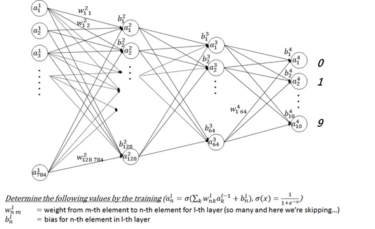
require(mxnet)###### read training data## train.csv is:# (label, pixel0, pixel1, ..., pixel783)# 1, 0, 0, ..., 0# 4, 0, 0, ..., 0# ...#####train <- read.csv("C:\tmp\train.csv", header=TRUE)train <- data.matrix(train)# separate label and pixeltrain.x <- train[,-1]train.y <- train[,1]# transform image pixel [0, 255] into [0,1]train.x <- t(train.x/255)# configure networkdata <- mx.symbol.Variable("data")fc1 <- mx.symbol.FullyConnected(data, name="fc1", num_hidden=128)act1 <- mx.symbol.Activation(fc1, name="relu1", act_type="relu")fc2 <- mx.symbol.FullyConnected(act1, name="fc2", num_hidden=64)act2 <- mx.symbol.Activation(fc2, name="relu2", act_type="relu")fc3 <- mx.symbol.FullyConnected(act2, name="fc3", num_hidden=10)softmax <- mx.symbol.SoftmaxOutput(fc3, name="sm")# train !# (If you want to use gpu, please set like ctx=list(mx.gpu(0),mx.gpu(1)) )mx.set.seed(0)model <- mx.model.FeedForward.create(  softmax,  X=train.x,  y=train.y,  ctx=mx.cpu(),  num.round=10,  array.batch.size=100,  learning.rate=0.07,  momentum=0.9,  eval.metric=mx.metric.accuracy,  initializer=mx.init.uniform(0.07),  epoch.end.callback=mx.callback.log.train.metric(100))###### read scoring data## test.csv is:# (pixel0, pixel1, ..., pixel783)# 0, 0, ..., 0# 0, 0, ..., 0# ...#####test <- read.csv("C:\tmp\test.csv", header=TRUE)test <- data.matrix(test)test <- t(test/255)# score !# ("preds" is the matrix of the possibility of each number)preds <- predict(model, test)###### output result (occurance count of each number)## The result is:#012 ... 9# 2814 3168 2711 ...  2778 #####pred.label <- max.col(t(preds)) - 1table(pred.label)

Here I don’t focus on the deep learning algorithms and networks itself, and you can proceed the rest of this readings as a black box for the details. I have briefly illustrated the network of this sample code as follows. (Here I don’t use any convolution layers and just use feed-forwarding.)
This sample is always fed forward without fed back or loops, and it’s resolved by the back-propagation algorithm (which determines the gradient) with 0.07 of learning rate (which is the ratio of delta for training) and 100 of batch size (which is the bunch of training data set for each time).

Setting up Spark clusters

As I described in my previous post, you can easily create your R Server and Spark clusters on Azure.
Here I skip how to setup, but please see my previous post for details (using Azure Data Lake store, RStudio setup, etc).

Moreover, here you have one more thing that needs to be done.
Currently R Server on Azure HDInsight (Hadoop) cluster is not including MXNet. Because of this reason, you must install MXNet on all worker nodes (ubuntu 16) using HDInsight script action. (You just only create the installation script and set this script on Azure Portal. See the following screenshot.)

Note : If you want to apply the script action on the edge node, you must use the sku of HDInsight Premium. So it’s better to run the MXNet workloads only on worker nodes. (The edge node is just for orchestrating.)

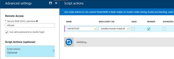
Below is my script action (.sh) for MXNet installation. Here we’re downloading the source code of MXNet and compiling with gcc.
As you can see, you don’t need to utilize GPU in scoring phase, and installation (compilation) is much simpler.

#!/usr/bin/env bash############ HDInsight script action# for installing MXNet# without GPU utilized############ install gcc, python libraries, etcsudo apt-get install -y libatlas-base-dev libopencv-dev libprotoc-dev python-numpy python-scipy make unzip git gcc g++ libcurl4-openssl-dev libssl-devsudo update-alternatives --install "/usr/bin/cc" "cc" "/usr/bin/gcc" 50MXNET_HOME="$HOME/mxnet/"# download MXNet source code (incl. dmlc-core, etc)git clone https://github.com/dmlc/mxnet.git "$HOME/mxnet/" --recursive# make and install MXNet and related modulescd "$MXNET_HOME"make -j$(nproc)sudo Rscript -e "install.packages('devtools', repo = 'https://cran.rstudio.com')"cd R-packagesudo Rscript -e "library(devtools); library(methods); options(repos=c(CRAN='https://cran.rstudio.com')); install_deps(dependencies = TRUE)"sudo Rscript -e "install.packages(c('curl', 'httr'))"sudo Rscript -e "install.packages(c('Rcpp', 'DiagrammeR', 'data.table', 'jsonlite', 'magrittr', 'stringr', 'roxygen2'), repos = 'https://cran.rstudio.com')"cd ..sudo make rpkgsudo R CMD INSTALL mxnet_current_r.tar.gz

Note : If your script action encounters some errors, you can see the log using Ambari UI https://{your cluster name}.azurehdinsight.net.

Prepare your trained model

Before running the scoring workloads, we prepare the trained model and save it to the local disk as follows. (See the following script.)
This script is saving the MXNet trained model in c:\tmp. Here the two of files, mymodel-symbol.json and mymodel-0100.params will be created.

Train and Save model for MNIST (R)

require(mxnet)###### train.csv is:# (label, pixel0, pixel1, ..., pixel783)# 1, 0, 0, ..., 0# 4, 0, 0, ..., 0# ...###### read input datatrain <- read.csv("C:\tmp\train.csv", header=TRUE)train <- data.matrix(train)# separate label and pixeltrain.x <- train[,-1]train.y <- train[,1]# transform image pixel [0, 255] into [0,1]train.x <- t(train.x/255)# configure networkdata <- mx.symbol.Variable("data")fc1 <- mx.symbol.FullyConnected(data, name="fc1", num_hidden=128)act1 <- mx.symbol.Activation(fc1, name="relu1", act_type="relu")fc2 <- mx.symbol.FullyConnected(act1, name="fc2", num_hidden=64)act2 <- mx.symbol.Activation(fc2, name="relu2", act_type="relu")fc3 <- mx.symbol.FullyConnected(act2, name="fc3", num_hidden=10)softmax <- mx.symbol.SoftmaxOutput(fc3, name="sm")# train !# (If you want to use gpu, please set like ctx=list(mx.gpu(0),mx.gpu(1)) )mx.set.seed(0)model <- mx.model.FeedForward.create(  softmax,  X=train.x,  y=train.y,  ctx=mx.cpu(),  num.round=10,  array.batch.size=100,  learning.rate=0.07,  momentum=0.9,  eval.metric=mx.metric.accuracy,  initializer=mx.init.uniform(0.07),  epoch.end.callback=mx.callback.log.train.metric(100))# save model to file# (created : mymodel-symbol.json, mymodel-0100.params)if(file.exists("C:\tmp\mymodel-symbol.json"))  file.remove("C:\tmp\mymodel-symbol.json")if(file.exists("C:\tmp\mymodel-0100.params"))  file.remove("C:\tmp\mymodel-0100.params")mx.model.save(  model = model,  prefix = "C:\tmp\mymodel",  iteration = 100)

After running this script, upload these model files (mymodel-symbol.json, mymodel-0100.params) into the downloadable location. (The scoring program will extract these files.)
In my example, I uploaded to Azure Data Lake store (adl://mltest.azuredatalakestore.net/dnndata folder) which is the same storage as the primary storage of Hadoop cluster.

R Script for scaling

It’s ready. Now let’s start the programming for scaling.

As I mentioned in my previous post, we can use “rx” prefixed ScaleR functions for Spark cluster scaling.

“So… we must rewrite all the functions with ScaleR functions !?”

Don’t worry ! Of course, not.
In this case, you can just use rxExec() function, which enables some bunch of codes to be distributed into the clusters in parallel.

Let’s see the following sample code. (As I described in my previous post, this code should be run on the edge node.)

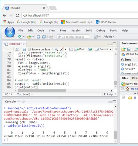
MNIST Scoring on Spark cluster (ML Server)

# Set Spark clusters contextspark <- RxSpark(  consoleOutput = TRUE,  extraSparkConfig = "--conf spark.speculation=true",  nameNode = "adl://mltest.azuredatalakestore.net",  port = 0,  idleTimeout = 90000)rxSetComputeContext(spark)image.score <- function(filename) {  require(mxnet)  storage.prefix <- "adl://mltest.azuredatalakestore.net/dnndata"#####  # test.csv is:  # (pixel0, pixel1, ..., pixel783)  # 0, 0, ..., 0  # 0, 0, ..., 0  # ...  #####  # copy model to local  if(file.exists("mymodel-symbol.json"))file.remove("mymodel-symbol.json")  if(file.exists("mymodel-0100.params"))file.remove("mymodel-0100.params")  rxHadoopCopyToLocal(file.path(storage.prefix, "mymodel-symbol.json"),"mymodel-symbol.json")  rxHadoopCopyToLocal(file.path(storage.prefix, "mymodel-0100.params"),"mymodel-0100.params")# load model  model_loaded <- mx.model.load(#prefix = "mymodel",prefix = "mymodel",iteration = 100  )  # copy scoring file to local  if(file.exists(filename))file.remove(filename)  srcfile <- file.path(storage.prefix, filename)  rxHadoopCopyToLocal(srcfile, filename)# read scoring data  #test <- read.csv(filename, header=TRUE)  test <- read.csv(filename,header=TRUE)  test <- data.matrix(test)  test <- t(test/255)# Score !  preds <- predict(model_loaded, test)  pred.label <- max.col(t(preds)) - 1  return(pred.label)}# FUN : function to execute in parallel# elemArgs : the arguments to the function# elemType : "nodes" or "cores"# timesToRun : total number of instances to runarglist <- list(  list(filename="test01.csv"),  list(filename="test02.csv"),  list(filename="test03.csv"),  list(filename="test04.csv"),  list(filename="test05.csv"),  list(filename="test06.csv"),  list(filename="test07.csv"),  list(filename="test08.csv"),  list(filename="test09.csv"),  list(filename="test10.csv"))result <- rxExec(  FUN = image.score,  elemArgs = arglist,  elemType = "nodes",  timesToRun = length(arglist))# output resultoutput <- table(unlist(result))print(output)

As you can see, here we are passing 10 “filename” arguments to image.score function using rxExec(). Eventually each image.score workloads (total 10 workloads) are distributed into the worker nodes on Spark cluster.
The return value of rxExec() is the aggregated results of 10 image.score instance executions.

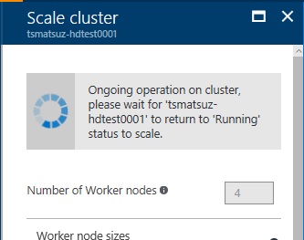
If needed, you can easily scale your cluster (ex. 4 nodes -> 16 nodes) on Azure Portal and get the massive computing resource for your workloads.

In “Channel9 – Deep Learning in Microsoft R Server Using MXNet on High-Performance GPUs in the Public Cloud“, they’re handling the real scenario of the CIFAR-10 image classification in Mona Lisa.

Azure Hadoop (Data Lake, HDInsight) team is also writing in the recent post for Caffe on Spark cluster, and please see, if you have much interest.

Azure Data Lake & Azure HDInsight Blog : Distributed Deep Learning on HDInsight with Caffe on Spark
https://blogs.msdn.microsoft.com/azuredatalake/2017/02/02/distributed-deep-learning-on-hdinsight-with-caffe-on-spark/

Note : With new rxExecBy(), you don’t have to manually split and move the data, and can be used on not only Spark cluster but any other parallel platforms. (Added on Apr 2017)