
Scale R workloads for machine learning (series)
- Statistical Machine Learning Workloads
- Deep Learning Workloads (Scoring phase)
- Deep Learning Workloads (Training phase) <– This post is here
In my previous post, I showed how to reduce your scoring workloads on deep learning using MXNetR.
Here I show how to accelerate (scaling up and out) in the training aspect on deep learning.
Get the power of devices – GPUs
For the training perspective, it needs so complicated calculations and so much computing workloads compared with the scoring workloads, and GPU is a very important factor for reducing and leveraging the workloads. (See the previous post. It needs to determine all the gradient, weights, and bias with the repeated matrices calculations.)
With MXNet, you can easily take advantage of GPU utilized deep learning, and let’s take a look at these useful capabilities.
First you can easily get the GPU utilized environment using Azure N-series (NC, NV) Virtual Machines. You must setup (install) all components (drivers, packages, etc) with the following installation script, and then you can get the GPU-powered MXNet. (You must compile MXNet with USE_CUDA=1 switch.) Because we’re setting up RStudio server as follows, you can connect to this Linux machine using your familiar RStudio client on the web.
For the details about this compiling, you can refer “Machine Learning team blog : Building Deep Neural Networks in the Cloud with Azure GPU VMs, MXNet and Microsoft R Server“.
I note that you should download the following software (drivers, tools) before running this script.
- CUDA local runfile from https://developer.nvidia.com/cuda-toolkit
(Here I’m using Ubuntu 16 with Intel architecture.) - cuDNN library for Linux from https://developer.nvidia.com/cudnn
(NVIDIA Developer registration is needed.) - MKL (Math Kernel Library) from https://software.intel.com/en-us/intel-mkl
(Intel Developer registration is needed.)
#!/usr/bin/env bash## install R (MRAN)#wget https://mran.microsoft.com/install/mro/3.3.2/microsoft-r-open-3.3.2.tar.gztar -zxvpf microsoft-r-open-3.3.2.tar.gzcd microsoft-r-opensudo ./install.sh -a -ucd ..sudo rm -rf microsoft-r-opensudo rm microsoft-r-open-3.3.2.tar.gz## install gcc, python, etc#sudo apt-get install -y libatlas-base-dev libopencv-dev libprotoc-dev python-numpy python-scipy make unzip git gcc g++ libcurl4-openssl-dev libssl-devsudo update-alternatives --install "/usr/bin/cc" "cc" "/usr/bin/gcc" 50## install CUDA (you can download cuda_8.0.44_linux.run)#chmod 755 cuda_8.0.44_linux.runsudo ./cuda_8.0.44_linux.run -overridesudo update-alternatives --install /usr/bin/nvcc nvcc /usr/bin/gcc 50export LIBRARY_PATH=/usr/local/cudnn/lib64/echo -e "export LIBRARY_PATH=/usr/local/cudnn/lib64/" >> .bashrc## install cuDNN (you can download cudnn-8.0-linux-x64-v5.1.tgz)#tar xvzf cudnn-8.0-linux-x64-v5.1.tgzsudo mv cuda /usr/local/cudnnsudo ln -s /usr/local/cudnn/include/cudnn.h /usr/local/cuda/include/cudnn.hexport LD_LIBRARY_PATH=/usr/local/cuda/lib64/:/usr/local/cudnn/lib64/:$LD_LIBRARY_PATHecho -e "export LD_LIBRARY_PATH=/usr/local/cuda/lib64/:/usr/local/cudnn/lib64/:$LD_LIBRARY_PATH" >> ~/.bashrc## install MKL (you can download l_mkl_2017.0.098.tgz)#tar xvzf l_mkl_2017.0.098.tgzsudo ./l_mkl_2017.0.098/install.sh# Additional setup for MRAN and CUDAsudo touch /etc/ld.so.confecho "/usr/local/cuda/lib64/" | sudo tee --append /etc/ld.so.confecho "/usr/local/cudnn/lib64/" | sudo tee --append /etc/ld.so.confsudo ldconfig## download MXNet source#MXNET_HOME="$HOME/mxnet/"git clone https://github.com/dmlc/mxnet.git "$HOME/mxnet/" --recursivecd "$MXNET_HOME"## configure MXNet#cp make/config.mk .# if use dist_sync or dist_async in kv_store (see later)#echo "USE_DIST_KVSTORE = 1" >>config.mk# if use Azure BLOB Storage#echo "USE_AZURE = 1" >>config.mk# For GPUecho "USE_CUDA = 1" >>config.mkecho "USE_CUDA_PATH = /usr/local/cuda" >>config.mkecho "USE_CUDNN = 1" >>config.mk# For MKL#source /opt/intel/bin/compilervars.sh intel64 -platform linux#echo "USE_BLAS = mkl" >>config.mk#echo "USE_INTEL_PATH = /opt/intel/" >>config.mk## compile and install MXNet#make -j$(nproc)sudo apt-get install libxml2-devsudo Rscript -e "install.packages('devtools', repo = 'https://cran.rstudio.com')"cd R-packagesudo Rscript -e "library(devtools); library(methods); options(repos=c(CRAN='https://cran.rstudio.com')); install_deps(dependencies = TRUE)"sudo Rscript -e "install.packages(c('curl', 'httr'))"sudo Rscript -e "install.packages(c('Rcpp', 'DiagrammeR', 'data.table', 'jsonlite', 'magrittr', 'stringr', 'roxygen2'), repos = 'https://cran.rstudio.com')"cd ..sudo make rpkgsudo R CMD INSTALL mxnet_current_r.tar.gzcd ..## install RStudio server#sudo apt-get -y install gdebi-corewget -O rstudio.deb https://download2.rstudio.org/rstudio-server-0.99.902-amd64.debsudo gdebi -n rstudio.debNote : Later I’ll explain about
USE_DIST_KVSTOREswitch.
“Still so much complicated and it takes much time to compile !”
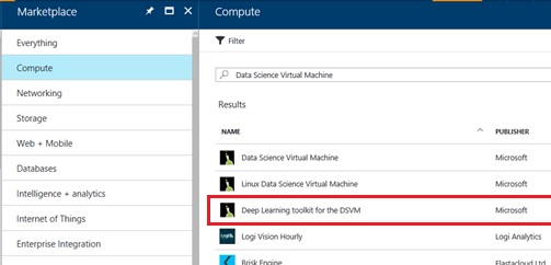
Don’t worry. If you think it’s hard, you can use pre-configured machines (VM) called “Deep Learning Toolkit for the DSVM (Data Science Virtual Machines)” in Microsoft Azure (see below). Using this VM template, you can take almost all components required for the deep neural network computing, including NC-series VM with GPUs (Telsa), those drivers (software and toolkit), Microsoft R, R Server, and GPU-accelerated MXNet (and other DNN libraries). No setup is needed with Azure !
I note that this deployment requires the access to Azure NC instances which depends on the choice the regions and HDD/SSD. In this post I selected South Central US region.
Note : Below is the matrix of available instance or services by Azure regions.
https://azure.microsoft.com/en-us/regions/services/
Here I’m using 2 GPUs labeled 0 and 1. (see below)
nvidia-smi -pm 1nvidia-smi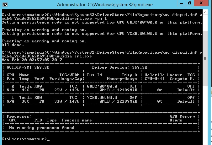
Now let’s see how it is used in our programming !
If you want to use GPUs for the training of neural networks, you can easily switch the device mode into GPU mode using MXNet as follows. In this code, the data batch is partitioned by 2 GPUs, and the results are summed up.
I note that here I don’t focus on the algorithms or networks itself (please refer the previous post) and I’m just using simple LeNet (Convolutional Neural Network, CNN) for MNIST dataset (which is the famous handwritten digits recognition example) to simplify our sample code. (This learning sample is not so deep (but shallow) and GPU power won’t be so much consumed (less than 10%) in this example.)
Please use more large data (like ImageNet dataset) or more deep-layred networks (like ResNet50) for benchmarking …
####### train.csv (training data) is:# (label, pixel0, pixel1, ..., pixel783)# 1, 0, 0, ..., 0# 4, 0, 0, ..., 0# ...######## test.csv (scoring data) is:# (pixel0, pixel1, ..., pixel783)# 0, 0, ..., 0# 0, 0, ..., 0# ...######require(mxnet)# read training datatrain <- read.csv( "C:\Users\tsmatsuz\Desktop\training\train.csv", header=TRUE)train <- data.matrix(train)# separate label and pixeltrain.x <- train[,-1]train.x <- t(train.x/255)train.array <- train.xdim(train.array) <- c(28, 28, 1, ncol(train.x))train.y <- train[,1]## configure network## inputdata <- mx.symbol.Variable('data')# first convconv1 <- mx.symbol.Convolution( data=data, kernel=c(5,5), num_filter=20)tanh1 <- mx.symbol.Activation( data=conv1, act_type="tanh")pool1 <- mx.symbol.Pooling( data=tanh1, pool_type="max", kernel=c(2,2), stride=c(2,2))# second convconv2 <- mx.symbol.Convolution( data=pool1, kernel=c(5,5), num_filter=50)tanh2 <- mx.symbol.Activation( data=conv2, act_type="tanh")pool2 <- mx.symbol.Pooling( data=tanh2, pool_type="max", kernel=c(2,2), stride=c(2,2))# first fullcflatten <- mx.symbol.Flatten(data=pool2)fc1 <- mx.symbol.FullyConnected( data=flatten, num_hidden=500)tanh3 <- mx.symbol.Activation( data=fc1, act_type="tanh")# second fullcfc2 <- mx.symbol.FullyConnected(data=tanh3, num_hidden=10)# losslenet <- mx.symbol.SoftmaxOutput(data=fc2)# train !kv <- mx.kv.create(type = "local")mx.set.seed(0)tic <- proc.time()model <- mx.model.FeedForward.create( lenet, X=train.array, y=train.y, ctx=list(mx.gpu(0),mx.gpu(1)), kvstore = kv, num.round=5, array.batch.size=100, learning.rate=0.05, momentum=0.9, wd=0.00001, eval.metric=mx.metric.accuracy, epoch.end.callback=mx.callback.log.train.metric(100))# score (1st time)test <- read.csv( "C:\Users\tsmatsuz\Desktop\training\test.csv", header=TRUE)test <- data.matrix(test)test <- t(test/255)test.array <- testdim(test.array) <- c(28, 28, 1, ncol(test))preds <- predict(model, test.array)pred.label <- max.col(t(preds)) - 1print(table(pred.label))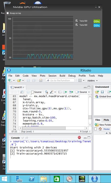
Distributed Training – Scale across multiple machines
MXNet training workload is not only distributed by devices (GPUs), but also multiple machines.
Here we assume there’re three machines (hosts), named “server01”, “server02”, and “server03”. Now we launch the parallel job on server02 and server03 from server01 console.
Before staring, you must compile MXNet with USE_DIST_KVSTORE=1 on all hosts. (See the above bash script example)
Note : Currently this distributed kvstore settings (
USE_DIST_KVSTORE=1) is not enabled in existing Data Science Virtual Machines (DSVM) or Deep Learning Toolkit for the DSVM by default. Hence you must setup (compile) by yourself.
In terms of the distribution protocol, ssh, mpi (mpirun), and yarn can be used for the remote execution and cluster management. Here we use ssh for example.
First we setup the trust between host machines.
We create the key pair on server01 using the following command, and the generated key pair (id_rsa and id_rsa.pub) is in .ssh folder. During creation, you set blank (null) to the certificate password (passphrase).
ssh-keygen -t rsals -al .sshdrwx------ 2 tsmatsuz tsmatsuz 4096 Feb 21 05:01 .drwxr-xr-x 7 tsmatsuz tsmatsuz 4096 Feb 21 04:52 ..-rw------- 1 tsmatsuz tsmatsuz 1766 Feb 21 05:01 id_rsa-rw-r--r-- 1 tsmatsuz tsmatsuz 403 Feb 21 05:01 id_rsa.pubNext you copy the generated public key (id_rsa.pub) into {home of the same user id}/.ssh directory on server02 and server03. The file name must be “authorized_keys“.
Now let’s confirm that you can pass the command (pwd) to the remote hosts (server02, server03) from server01 as follows. If succeeded, the current working directory on remote host will be returned. (We assume that 10.0.0.5 is the ip address of server02 or server03.)
ssh -o StrictHostKeyChecking=no 10.0.0.5 -p 22 pwd/home/tsmatsuzNext you create the file named “hosts” in your working directory on server01, and please write the ip of accessing remote hosts (server02 and server03) in each rows.
10.0.0.510.0.0.6In my example, I simply use the following trainig script test01.R (which is executed on remote hosts). As you can see, here we set the dist_sync for kvstore value, which means the synchronous parallel execution. (The weight and bias on remote hosts will be updated synchronously.)
test01.R
####### train.csv (training data) is:# (label, pixel0, pixel1, ..., pixel783)# 1, 0, 0, ..., 0# 4, 0, 0, ..., 0# ...######## test.csv (scoring data) is:# (pixel0, pixel1, ..., pixel783)# 0, 0, ..., 0# 0, 0, ..., 0# ...######require(mxnet)# read training datatrain_d <- read.csv( "train.csv", header=TRUE)train_m <- data.matrix(train_d)# separate label and pixeltrain.x <- train_m[,-1]train.y <- train_m[,1]# transform image pixel [0, 255] into [0,1]train.x <- t(train.x/255)# configure networkdata <- mx.symbol.Variable("data")fc1 <- mx.symbol.FullyConnected(data, name="fc1", num_hidden=128)act1 <- mx.symbol.Activation(fc1, name="relu1", act_type="relu")fc2 <- mx.symbol.FullyConnected(act1, name="fc2", num_hidden=64)act2 <- mx.symbol.Activation(fc2, name="relu2", act_type="relu")fc3 <- mx.symbol.FullyConnected(act2, name="fc3", num_hidden=10)softmax <- mx.symbol.SoftmaxOutput(fc3, name="sm")# train !model <- mx.model.FeedForward.create( softmax, X=train.x, y=train.y, ctx=mx.cpu(), num.round=10, kvstore = "dist_sync", array.batch.size=100, learning.rate=0.07, momentum=0.9, eval.metric=mx.metric.accuracy, initializer=mx.init.uniform(0.07), epoch.end.callback=mx.callback.log.train.metric(100))Now you can run the parallel execution.
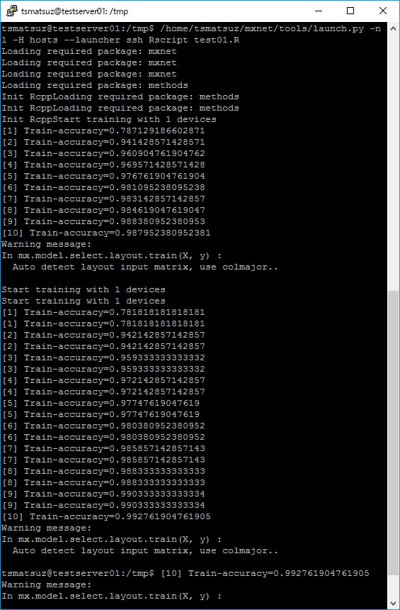
On server01 console, you call the following launch.py with executable command “Rscript test01.R“. Then this command is executed on server02 and server03, and those are traced by the job monitor. (Here we assume that /home/tsmatsuz/mxnet is the installation directory of MXNet.)
Note that be sure to put this R script (test01.R) and the training data (train.csv) in the same directory on server02 and server03. If you want to see the weight and bias are properly updated, it’s better to use the different training data between server02 and server03. (Or it’ll be better to download appropriate data files from remote site on the fly.)
/home/tsmatsuz/mxnet/tools/launch.py -n 1 -H hosts --launcher ssh Rscript test01.RThe output result is the following. The upper side is the result by the single node, and bottom side is the synchronized result by server02 and server03.
Note : In your real application, it’s better to use the InfiniBand network. Sorry, but please be patient to be released InfiniBand support on Azure VM N-series.
Appendix : Incremental Training with MXNet
As you know, it will take much wasting time to re-train from the beginning. With MXNet, you can also save the trained model, and refine the model incrementally with new data as follows.
As you can see below (see bold fonts), we’re setting the previously trained symbol and parameters in the 2nd training.
####### train.csv (training data) is:# (label, pixel0, pixel1, ..., pixel783)# 1, 0, 0, ..., 0# 4, 0, 0, ..., 0# ...######## test.csv (scoring data) is:# (pixel0, pixel1, ..., pixel783)# 0, 0, ..., 0# 0, 0, ..., 0# ...######require(mxnet)# read first 500 training datatrain_d <- read.csv( "C:\Users\tsmatsuz\Desktop\training\train.csv", header=TRUE)train_m <- data.matrix(train_d[1:500,])# separate label and pixeltrain.x <- train_m[,-1]train.y <- train_m[,1]# transform image pixel [0, 255] into [0,1]train.x <- t(train.x/255)# configure networkdata <- mx.symbol.Variable("data")fc1 <- mx.symbol.FullyConnected(data, name="fc1", num_hidden=128)act1 <- mx.symbol.Activation(fc1, name="relu1", act_type="relu")fc2 <- mx.symbol.FullyConnected(act1, name="fc2", num_hidden=64)act2 <- mx.symbol.Activation(fc2, name="relu2", act_type="relu")fc3 <- mx.symbol.FullyConnected(act2, name="fc3", num_hidden=10)softmax <- mx.symbol.SoftmaxOutput(fc3, name="sm")# train !model <- mx.model.FeedForward.create( softmax, X=train.x, y=train.y, ctx=mx.cpu(), num.round=10, array.batch.size=100, learning.rate=0.07, momentum=0.9, eval.metric=mx.metric.accuracy, initializer=mx.init.uniform(0.07), epoch.end.callback=mx.callback.log.train.metric(100))# score (1st time)test <- read.csv("C:\Users\tsmatsuz\Desktop\training\test.csv", header=TRUE)test <- data.matrix(test)test <- t(test/255)preds <- predict(model, test)pred.label <- max.col(t(preds)) - 1table(pred.label)## save the current model if needed## save model to filemx.model.save( model = model, prefix = "mymodel", iteration = 500)# load model from filemodel_loaded <- mx.model.load( prefix = "mymodel", iteration = 500)# re-train for the next 500 data !train_d <- read.csv( "C:\Users\tsmatsuz\Desktop\training\train.csv", header=TRUE)train_m <- data.matrix(train_d[501:1000,])train.x <- train_m[,-1]train.y <- train_m[,1]train.x <- t(train.x/255)model = mx.model.FeedForward.create( model_loaded$symbol, arg.params = model_loaded$arg.params, aux.params = model_loaded$aux.params, X=train.x, y=train.y, ctx=mx.cpu(), num.round=10, #kvstore = kv, array.batch.size=100, learning.rate=0.07, momentum=0.9, eval.metric=mx.metric.accuracy, initializer=mx.init.uniform(0.07), epoch.end.callback=mx.callback.log.train.metric(100))# score (2nd time)test <- read.csv("C:\Users\tsmatsuz\Desktop\training\test.csv", header=TRUE)test <- data.matrix(test)test <- t(test/255)preds <- predict(model, test)pred.label <- max.col(t(preds)) - 1table(pred.label)Note : So much training doesn’t necessarily generate a good model. Please see “Overfitting in Regression and Neural Nets” and estimate your model with validation (unknown) dataset.
[Reference] MXNet Docs : Run MXNet on Multiple CPU/GPUs with Data Parallel
http://mxnet.io/how_to/multi_devices.html
Categories: Uncategorized
