Quantum Fourier Transform & Quantum Phase Estimation (Q#)

By Tsuyoshi Matsuzaki on 2019-04-26• ( 4 Comments )

(Download source code from here.)

In this post, I’ll explain quantum algorithms of Quantum Phase Estimation with Q# implementation.

Series : Quantum algorithm’s implementation (Q#)

Quantum Fourier Transform (QFT)

Before describing the idea of Quantum Phase Estimation, let me start with Quantum Fourier Transform (QFT), which is the quantum state’s unitary transformation defined as below :

$\displaystyle \left| x \right> \to \frac{1}{\sqrt{2^n}} \sum_{k=0}^{2^n - 1} e^{2 \pi i x k / 2^n} \left| k \right>$

For arbitrary states $\sum_x b_x \left| x \right>$ in general, this transformation can be written as :

$\displaystyle \sum_x b_x \left| x \right> \to \frac{1}{\sqrt{2^n}} \sum_{k=0}^{2^n - 1} \sum_x b_x e^{2 \pi i x k / 2^n} \left| k \right>$

If you’re familiar with classical Discrete Fourier Transform, you will find this QFT (Quantum Fourier Transform) has the same form and keeps the same characteristics, such as linearity, pairwise products, and invertibility.
The classical one is used for finding time-based sine waves, and QFT can also be used for the same purpose as follows.

$\displaystyle \frac{1}{\sqrt{2^2}} \left| 00 \right> - \frac{1}{\sqrt{2^2}} \left| 01 \right> + \frac{1}{\sqrt{2^2}} \left| 10 \right> - \frac{1}{\sqrt{2^2}} \left| 11 \right>$

$\displaystyle \to \frac{1}{\sqrt{2^2}} \sum_{k=0}^{2^2 - 1} \left( \frac{1}{\sqrt{2^2}} e^{2\pi i \times 0 \times k / 2^2} \left| k \right> - \frac{1}{\sqrt{2^2}} e^{2\pi i \times 1 \times k / 2^2} \left| k \right> + \frac{1}{\sqrt{2^2}} e^{2\pi i \times 2 \times k / 2^2} \left| k \right> - \frac{1}{\sqrt{2^2}} e^{2\pi i \times 3 \times k / 2^2} \left| k \right> \right)$

$\displaystyle = \frac{1}{2} \sum_{k=0}^{3} \left( \frac{1}{2} \left| k \right> - \frac{1}{2} e^{\frac{\pi i k}{2}} \left| k \right> + \frac{1}{2} e^{\frac{2 \pi i k}{2}} \left| k \right> - \frac{1}{2} e^{\frac{3 \pi i k}{2}} \left| k \right> \right)$

$\displaystyle = \frac{1}{2} \left( \frac{1}{2} \times 0 \cdot \left| 00 \right> + \frac{1}{2} \times 0 \cdot \left| 01 \right> + \frac{1}{2} \times 4 \cdot \left| 10 \right> + \frac{1}{2} \times 0 \cdot \left| 11 \right> \right)$

$\displaystyle = \left| 10 \right>$

It’s known that Quantum Fourier Transform (QFT) can be implemented by the following circuit, where $\left| x \right> = \left| x_0 \right> \left| x_1 \right> \ldots \left| x_{n-1} \right>$ . I don’t describe why this circuit realizes QFT, but the proof is well-described in the lecture “Chem/CS/Phys191: Qubits, Quantum Mechanics, and Computers – Quantum Fourier Transform (UC Berkeley)” if you’re interested.
Note that the last part of SWAP can be implemented by n / 2 times combination of 2 bit’s SWAP : $(SWAP)_{1 2} = (CNOT)_{1 2} (CNOT)_{2 1} (CNOT)_{1 2}$ . (As I’ll show you later, we use Q# function Microsoft.Quantum.Canon.SwapReverseRegister() for this operation in this post.)

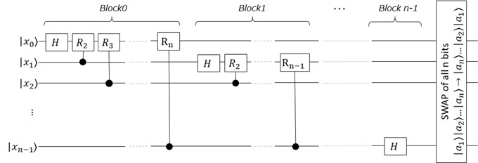
where $\displaystyle R_k = \begin{pmatrix} 1$

Figure 01 : Quantum Fourier Transform (QFT)

Quantum Phase Estimation

As you will find in this post, QFT will help you to find phase in quantum state (i.e, quantum phase estimation), and it can also be applied for more advanced algorithms, such as, Shor’s algorithm (which I will discuss in the future post).
Now let me start to explain the idea of Quantum Phase Estimation, using QFT.

Here we assume that some state $\left| \psi \right>$ is represented by the following $0 \leq \phi < 2 \pi$ . Here $\left| \psi \right>$ is given, but $\phi$ is unknown.

$\left| \psi \right> = \displaystyle \frac{1}{2^n} \sum_{k=0}^{2^n - 1} e^{i \phi k} \left| k \right>$

The goal of Phase Estimation is to find the unknown $\phi$ using state $\left| \psi \right>$ .

Note : See here for quantum phase in 2 state system.

As you can easily see, if $\phi$ is written as $\phi = 2 \pi a / 2^n$ for some integer “ $a$ “, this equation is the same as the right side of QFT. Then hopefully we might get integer “ $a$ ” (eventually, the result $\phi$ ) by $QFT^{-1}$ transformation (running QFT circuit from backwards) and measuring the result’s integer. (For instance, if $QFT^{-1} \left| \psi \right> = \left| 0 \right>\left| 1 \right>\left| 1 \right> = \left| 011 \right>$ , we can expect that the integer “a” results into $0 \times 2^2 + 1 \times 2^1 + 1 \times 2^0 = 3$ .)
Here I skip the proof, but it’s known that you can get the approximate integer “ $a$ ” (i.e, it holds $\phi \fallingdotseq 2 \pi a / 2^n$ ) by $QFT^{-1}$ with high probabilities, even if it’s not precise $\phi = 2 \pi a / 2^n$ . That is, even if $\phi = 2 \pi (a/2^n + \delta)$ with some error $0 \leq | \delta | \leq 1/2^{n+1}$ , you can get the approximate integer part “ $a$ ” with high probability by $QFT^{-1}$ .
When $n$ increases, you will get more accurate $\phi \fallingdotseq 2 \pi a / 2^n$ with the estimated integer value “ $a$ “.

Note : If you’re interested in the proof of this approximation, you can refer “Principles of Quantum Computation and Information“. (See Volume 1 – Chapter 3.12 “Quantum phase estimation”.)

This algorithm can also be applied to the following another problem.
Here we assume we have a given unitary $U$ and eigenstate $\left| u \right>$ . $U$ is unitary, then corresponding eigenvalue is written as $e^{i\phi}$ for some $0 \leq \phi < 2 \pi$ . Now we want to find this $\phi$ using a given $U$ and $\left| u \right>$ .

Because of $U \left| u \right> = e^{i\phi} \left| u \right>$ , you can find $U^r \left| u \right> = (e^{i\phi})^r \left| u \right>$ (where r is integer).
Now we consider Controlled- $U^{2^j}$ operation (where j is integer), in which we apply $U^{2^j}$ to the second qubit, conditional on the first qubit. We then apply this operation to $1/\sqrt{2}(\left| 0 \right> + \left| 1 \right>) \left| u \right>$ as follows. :

$\verb|Controlled-| U^{2^j} : \frac{1}{\sqrt{2}}(\left| 0 \right> + \left| 1 \right>) \left| u \right> \rightarrow \frac{1}{\sqrt{2}}(\left| 0 \right> \left| u \right> + \left| 1 \right> U^{2^j} \left| u \right>) = \frac{1}{\sqrt{2}}(\left| 0 \right> + e^{i2^j \phi} \left| 1 \right>) \left| u \right>$

Note : Here, we can get the first qubit by $H \left| 0 \right> = 1/\sqrt{2}(\left| 0 \right> + \left| 1 \right>)$ .

Now let’s expand this transformation to arbitrary $m$ dimension, and see the following circuit.
In this circuit, $m$ is the dimension of eigenvector $\left| u \right>$ and $n$ is an arbitrary integer. (i.e, $m=2^q$ where q is the number of qubits $\left| u \right>$ , and $U$ is then represented by $m \times m$ unitary matrix.)

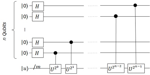
Figure 2 : Transform with n register qubits

By the previous equation, this circuit (Figure 2) will generate the following states :

$\displaystyle \frac{1}{\sqrt{2^n}} (\left| 0 \right> + e^{i2^{n-1} \phi} \left| 1 \right>) \ldots (\left| 0 \right> + e^{i2 \phi} \left| 1 \right>) (\left| 0 \right> + e^{i \phi} \left| 1 \right>) \left| u \right> \\ = \frac{1}{2^n} \sum_{k = 0}^{2^n - 1} e^{i \phi k} \left| k \right> \left| u \right>$

As you can see in the right side of this equation, the representation of this first $2^n$ qubits (i.e, $\left| k \right>$ ) is the same formula as previous phase estimation problem. You can then find $\phi$ by applying $QFT^{-1}$ for the first $2^n$ qubits.

As a result, you can estimate eigenvalue with the following circuit.

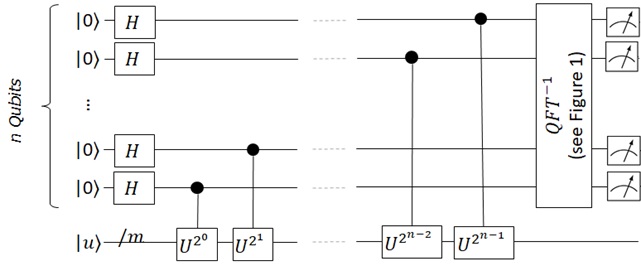
Figure 3 : Eigenvalue Estimation

By the way, recall that $n$ is an arbitrary integer. How large should we set for $n$ in this circuit ?
As I have mentioned above, you can get more accurate approximate value by increasing this $n$ . But if you increase $n$ more and more, the complexity (the cost) of this phase estimation will increase rapidly (exponentially), as above circuit shows.
Therefore you must carefully set $n$ to meet the requirements between cost (complexity) and accuracy in quantum phase estimation algorithm.

Q# Programming for Quantum Phase Estimation

In this post, I’ll implement eigenvalue estimation for a given $U$ and eigenstate $\left| u \right>$ .

To simplify our example, we assume that the following unitary operator $U$ is given as a black-box oracle operator. (As you can see later, this is easily implemented by Rz() operator in Q#.) :

$\displaystyle \begin{pmatrix} e^{-i\theta / 2}$

As you can easily see, this unitary operator has eigenvalues : $e^{i\theta / 2}$ and $e^{-i\theta / 2}$ , and corresponding eigenstates : $\left| 1 \right>$ and $\left| 0 \right>$ . In this example, we give a eigenstate $\left| 1 \right>$ and try to estimate eigenvalue $e^{i\theta / 2}$ .

Note : Phase Estimation example in official GitHub repo uses Faster Phase Estimation (not Quantum Phase Estimation), which is the optimized iterative phase estimation algorithm based on the classical post-processing ideas. For Faster Phase Estimation, please see this paper by Microsoft Research.
In this post, we show you Quantum Phase Estimation (above algorithm) by QFT.

Now let’s start our programming.

In fact, Q# provides high-level operator (in Microsoft.Quantum.Standard) for both Quantum Fourier Transform (QFT) and Phase Estimation, and you don’t need to implement these algorithms by yourself. (See QFT() and QuantumPhaseEstimation() in the reference document.)
But here, let me implement these algorithms with primitive operators for the purpose of your learning.

First we implement QFT (see Figure 1 above) as follows.
As I have mentioned above, you can implement the swap operation for all qubits by $2/n$ combinations of 3 CNOT gates, but here I have used Microsoft.Quantum.Canon.SwapReverseRegister() for simplifying our sample code.

operation QFTImpl (qs : Qubit[]) : Unit is Adj + Ctl{  body (...)  {let nQubits = Length(qs);  for i in 0 .. nQubits - 1{  H(qs[i]);  for j in i + 1 .. nQubits - 1  {Controlled R1Frac([qs[j]], (1, j - i, qs[i]));  }}  Microsoft.Quantum.Canon.SwapReverseRegister(qs);  }}

Next we implement quantum eigenvalue estimation algorithm described in above Figure 3. (This logic (circuit) invokes $QFT^{-1}$ as follows.)
Here the argument “oracle” is a black-box unitary operator $U$ , and “targetState” is corresponding eigenstate, and “controlRegister” is $n$ register qubits in Figure 3.

operation QuantumPhaseEstimationImpl (oracle : (Qubit[] => Unit is Adj + Ctl), targetState : Qubit[], controlRegister : Qubit[]) : Unit is Adj + Ctl{  body (...)  {let nQubits = Length(controlRegister);Microsoft.Quantum.Canon.ApplyToEachCA(H, controlRegister);  for idxControlQubit in 0 .. nQubits - 1{  let control = (controlRegister)[nQubits - 1 - idxControlQubit];  let power = 2 ^ idxControlQubit;  Controlled PowerOracle([control], (oracle, targetState, power));  //// You can also write as follows,  //// Or use Microsoft.Quantum.Canon.DiscreteOracle instead  //for idxPower in 0 .. power - 1  //{  //  Controlled oracle([control], targetState);  //}}Adjoint QFTImpl(controlRegister);  }}operation PowerOracle (oracle : (Qubit[] => Unit is Adj + Ctl), targetState : Qubit[], power : Int) : Unit is Adj + Ctl {  body (...) {for idxPower in 0 .. power - 1{  oracle(targetState);}  }}

Now we define a black-box unitary (oracle) $U$ as follows.
As I have mentioned above, this eigenvalue (corresponding eigenvector $\left| 1 \right>$ ) is $e^{i\theta / 2}$ .
Then our goal is to estimate the following “eigenphase” (i.e, $\theta$ ) .

operation ExpOracle (eigenphase : Double, register : Qubit[]) : Unit is Adj + Ctl {  body (...) {Rz(2.0 * eigenphase, register[0]);  }}

Now we combine these operators.
First we generate ExpOracle() (i.e, $U$ ) with some eigenphase.
Next we prepare eigenstate $\left| 1 \right>$ and $n$ register qubits.
Finally we execute estimation by calling QuantumPhaseEstimationImpl().

For simplification, I have used Microsoft.Quantum.Arithmetic.MeasureInteger() for getting measured integer, but you can easily implement the same logic by measuring each register qubits and sum all bits as binary number.

Note (BigEndian and LittleEndian) :
For instance, the measured integer of $\left| 011 \right>$ (1st qubit is 0 and others are 1) becomes 3 when you use Big Endian (BigEndian). However, it becomes $110_{(2)} = 6$ when you use Little Endian (LittleEndian).
In our case, we need Big Endian.

operation PhaseEstimationSample (eigenphase : Double) : Double {  let oracle = ExpOracle(eigenphase, _); // Generate (Qubit[] => Unit) with eigenphase   let n = 10;  mutable estPhase = 0.0;  use (eigenstate, phaseRegister) = (Qubit[1], Qubit[n]) {X(eigenstate[0]);QuantumPhaseEstimationImpl(oracle, eigenstate, phaseRegister);let estReg = Microsoft.Quantum.Arithmetic.MeasureInteger(  Microsoft.Quantum.Arithmetic.BigEndianAsLittleEndian(Microsoft.Quantum.Canon.BigEndian(phaseRegister)));set estPhase = 2.0 * PI() * IntAsDouble(estReg) / IntAsDouble(2 ^ n);Reset(eigenstate[0]);  }  return estPhase;}

Now let’s invoke quantum logic from Python or .NET (C#).

import randomrandom.seed(1000)eigenphase = random.uniform(0.0, 1.0) * 3.0 * 2.0est = PhaseEstimationSample.simulate(eigenphase=eigenphase)print("expected {}, estimated {}".format(eigenphase, est))eigenphase = random.uniform(0.0, 1.0) * 3.0 * 2.0est = PhaseEstimationSample.simulate(eigenphase=eigenphase)print("expected {}, estimated {}".format(eigenphase, est))eigenphase = random.uniform(0.0, 1.0) * 3.0 * 2.0est = PhaseEstimationSample.simulate(eigenphase=eigenphase)print("expected {}, estimated {}".format(eigenphase, est))

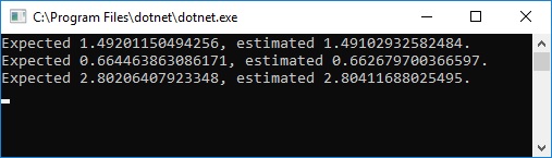
You will then get the following results and find that the phase ( $\theta$ ) is well-estimated by algorithm.

You can download and run this source code from here.

In previous posts, we saw phase kickback method in quantum, which is used in several primitive algorithms for black-box problems.
As you saw above, Quantum Fourier Transform (QFT) translates a bit shift into phase shifts, which can be used in more advanced algorithms, such as, Quantum Phase Estimation.

In the next post, I will introduce several basic quantum operations for the preparation of famous Shor’s algorithm.

Reference :

Principles of Quantum Computation and Information

Categories: Uncategorized

Tagged as: Quantum

tsmatz

Professional Development, Data Science

Quantum Fourier Transform & Quantum Phase Estimation (Q#)

Quantum Fourier Transform (QFT)

Quantum Phase Estimation

Q# Programming for Quantum Phase Estimation

4 replies»

Leave a Reply Cancel reply

Recent Posts

Reinforcement Learning

Imitation Learning

Language Processing

Diffusion Models

Tags

Follow

Quantum Fourier Transform & Quantum Phase Estimation (Q#)

Quantum Fourier Transform (QFT)

Quantum Phase Estimation

Q# Programming for Quantum Phase Estimation

Share this:

Related

4 replies»

Leave a Reply Cancel reply

Recent Posts

Reinforcement Learning

Imitation Learning

Language Processing

Diffusion Models

Tags

Follow