Introduce Time Series Analysis with ARIMA (Part 1)

By Tsuyoshi Matsuzaki on 2017-07-26• ( 3 Comments )

The time series analysis is frequently used in practice – such as, marketing analysis, stock analysis, social analysis, or log analysis.
In the series of posts (part 1 and part 2), I deal with ARIMA time series analysis.

To make you understand clearly, I’ll progress topics step-by-step – by discussing AR, MA, ARMA, ARIMA and seasonal ARIMA respectively as follows.

Table of Contents

Part 1 : AR, MA, ARMA (Stationary Model) <- this post
- Before I start … (Preface)
- What is AR, MA, and ARMA
- Find Model in Stationarity
- Estimate Parameters (in Stationary Model)
- Forecasting ARMA Time Series
Part 2 : ARIMA, Seasonal ARIMA (Non-Stationary Model)
- Non-Stationary Time Series (Introduction of ARIMA)
- Estimate Model and Forecast in ARIMA
- Backshift Notation
- Seasonal ARIMA (SARIMA)
- Find Seasonality

0. Before I start …

Understanding mathematics behind ARIMA is very important to exactly know time series analysis. From this perspective, this post will also help you to learn these mathematical ideas. (In order to focus on building your intuitions, I’ll explain mathematical ideas behind things without difficult descriptions or mathematical proofs as possible.)

I’ll also show you several example code to help you understand in R programming language.
Even when you’re not familiar with R, you might be able to easily understand these examples, because I’ll keep my source code as simple as possible throughout these posts.

Note : There also exist several other models for time series analysis – such like, GARCH, exponential smoothing, RNN-based modeling (deep learning), and so on. (See “Time Series Forecasting Best Practices“.)
For related topics, see “GitHub : Hidden Markov Models (HMM) and Linear Dynamical Systems (LDS)” for Python examples in sequential data with Markov chains.

1. What is AR, MA, and ARMA

First, I’ll introduce time series under stationary condition, ARMA (not ARIMA).
As you will find in the next post, the idea of ARIMA is based on this ARMA model. I’ll thus proceed to ARIMA, after you have well learned stationary model, ARMA.

Suppose, $\{y_t\}_{t=-\infty}^\infty$ is time series depending on time $t$ .
In this assumption, the “stationarity” (stationary process) in time series is defined as follows :

The mean value (expected value) at each time $t$ doesn’t depend on time $t$ . (It’s a constant $\mu$ in any time $t$ .)
The autocovariance $Cov(y_{t_1},y_{t_2})$ (i.e, $E\left[(y_{t_1} - E[y_{t_1}]) (y_{t_2} - E[y_{t_2}])\right]$ , where $E[]$ is a mean) only depends on the time lag $t_1 - t_2$ , not depends on time $t_1, t_2$ .

The stationary process is then written as the following equation for any time lag (interval) $k$ :

$\displaystyle E[y_t] = E[y_{t-k}] = \mu$

$\displaystyle Cov(y_t, y_{t-k}) = \gamma(k)$

where $\gamma(k)$ is some function only depending on $k$ .

Note : Strictly speaking, the above is called “weak-sense stationary process”. This definition is often used rather than “strongly stationary process” in practice.
Through this series of posts, I assume “weak-sense stationarity”, when I use the term “stationarity”.
See “Stationary process (Wikipedia)“.

Intuitively it means : the stochastic behavior of value’s motion is always same in any time $t$ .
For a brief example, it is not stationary process, if values increase more and more as time passes. (Because the mean is not constant and depends on $t$ .)

Now I will proceed to AR, MA, and ARMA models based on this assumption.
To make you have a clear picture, let’s consider the stock price data. (Note that the real stock price data would be non-stationary, but here I suppose it’s stationary.)
As you know, the stock price will be influenced by the yesterday’s price. If the price (stock closing price) of $t - 1$ is $y$ dollars, the price of day $t$ will start with $y$ dollars.
We can then assume that the price $y_t$ at day $t$ will hold the following equation. :

$\displaystyle y_t = c + \phi y_{t-1} + \epsilon_t$

where $c$ and $\phi$ are constant values, and $\{\epsilon_t\}$ is randomly distributed noise data called “white noise”.
Here both mean and autocovariance of $\{\epsilon_t\}_{t=-\infty}^\infty$ equal to $0$ , and you can then suppose $\{\epsilon_t\}_{t=-\infty}^\infty$ as $\mathcal{N}(0, \sigma^2)$ to simplify.

Note : If $\phi$ is negative value, $y_t$ has the reverse correlation of $y_{t-1}$ . (When $y_{t-1}$ is large, $y_t$ will be negatively large.)
In this case, the curve of this series will be so jagged.

This model is called AR (Autoregressive).
In general, AR(p) is given as the following definition. (Therefore the above stock model is denoted as AR(1).)

$\displaystyle y_t = c + \phi_1 y_{t-1} + \phi_2 y_{t-2} + \cdots + \phi_p y_{t-p} + \epsilon_t\;\;({}^{\forall}t)$

Note : In directed graphical model (Bayesian networks), AR is the model, in which each node has a Gaussian distribution whose mean is a linear function of its parents.
There exists an alternative approach (tapped delay line, TDL) to use neural networks instead of linear-Gaussian models.

This AR model can represent many aspects of cyclic stationarity.
For example, the following R program will plot AR(2) with $\phi_1 = 1.8,\phi_2 = -0.9$ . As you can see below, the curve for this data will show some cycles.

data_count <- 300cons <- 70y1 <- 10phi1 <- 1.8phi2 <- -0.9e <- rnorm(data_count) * 10y2 <- cons + (phi1 * y1) + e[2]y <- data.frame(  Indexes=c(1, 2),  Values=c(y1, y2))for (i in 3:data_count) {  yi <- cons + (phi1 * y$Values[i-1]) + (phi2 * y$Values[i-2]) + e[i]  y <- rbind(y,data.frame(Indexes=c(i), Values=c(yi)))}plot(y)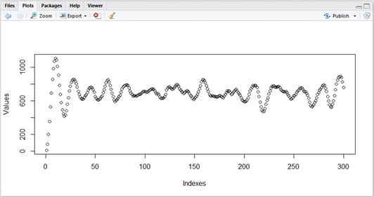

Note : You can simply use the function arima.sim() (in stats package) for ARIMA model simulation. (In this post, I didn’t use this function for your understanding.)
Note : Throughout this post, I don’t care the index of time – such as “day of month”, “day of week”, “quarter” – to simplify examples.
If you want to handle these time signatures, timekit package in R will help you.

Remember that not all AR expression is stationary process. AR model has the stationarity, only if some condition is established.
For instance, in AR(1), it has stationarity if and only if $| \phi_1 | < 1$ .
In AR(2), it has stationarity if and only if $\phi_2 > -1,\phi_2 < 1 + \phi_1$ and $\phi_2 < 1 - \phi_1$ .

Now let’s proceed to MA part.
The stock price might also be affected by the difference between yesterday’s open price and closing price. For instance, if the stock price rapidly decreases on the day $t$ , the price might rebound on the day $t + 1$ .
In such a case, we can consider the following model called MA (moving average).

$\displaystyle y_t = \mu + \epsilon_t + \theta \epsilon_{t-1}$

The part of $\mu + \epsilon_t$ ( $\mu$ is the mean) is the same like $c + \epsilon_t$ in AR, but MA depends on noise $\epsilon_{t-1}$ , instead of $y_{t-1}$ .

Same as AR, the general MA(q) representation is given as following equation.
It is known that MA(q) is always stationary process.

$\displaystyle y_t = \mu + \epsilon_t + \theta_{t-1} \epsilon_{t-1} + \theta_{t-2} \epsilon_{t-2} + \cdots + \theta_{t-q} \epsilon_{t-q} \;\;({}^{\forall}t)$

Let’s see how the curve will change with $\theta$ values.
As you can see below, it will smoothly transit, when $\theta$ is positively connected between $\theta_1, \theta_2, \ldots$ . On contrary, it will be jagged, when it’s negatively connected between $\theta_1, \theta_2, \ldots$ .

Normal Distribution (No MA)

MA(3) with $\theta_1 = 1,\theta_2 = 1,\theta_3 = 1$

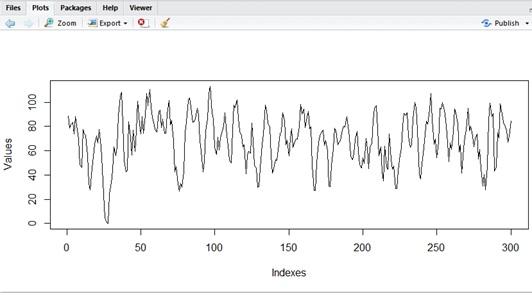
MA(2) with $\theta_1 = -1,\theta_2 = 1$

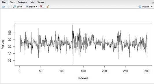
# Source code for curvedata_count <- 300mu <- 70# sample1#theta1 <- 0#theta2 <- 0#theta3 <- 0# sample2theta1 <- 1theta2 <- 1theta3 <- 1# sample3#theta1 <- -1#theta2 <- 1#theta3 <- 0e <- rnorm(data_count) * 10y1 <- mu + e[1]y2 <- mu + e[2] + (theta1 * e[1])y3 <- mu + e[3] + (theta1 * e[2]) + (theta2 * e[1])y <- data.frame(  Indexes=c(1, 2, 3),  Values=c(y1, y2, y3))for (i in 4:data_count) {  yi <- mu + e[i] + (theta1 * e[i-1]) + (theta2 * e[i-2]) + (theta3 * e[i-3])  y <- rbind(y,data.frame(Indexes=c(i), Values=c(yi)))}plot(y, type="l")

Finally, the combined model between AR and MA is called ARMA model, and it’s given as follows.
As you can see below, the former part is AR(p) and the latter is MA(q).

$\displaystyle y_t = c + \phi_1 y_{t-1} + \phi_2 y_{t-2} + \cdots + \phi_p y_{t-p} + \epsilon_t + \theta_{t-1} \epsilon_{t-1} + \theta_{t-2} \epsilon_{t-2} + \cdots + \theta_{t-q} \epsilon_{t-q}\;\;({}^{\forall}t)$

2. Find Model in Stationarity

Now I’ll proceed to the prediction for given time series data (stationary data).
However, before prediction, we should find the appropriate model and parameters – $p, q, \theta, \phi, \ldots$
In order to identify model (AR, MA, or ARMA) and dimensions ( $p$ and $q$ ), I’ll focus on the characteristics of each models – AR, MA, and ARMA. As you’ll find in this section, each model has the different characteristics for autocorrelation (ACF) and partial autocorrelation (PACF).

First, autocorrelation (shortly, Corr) is the autocovariance divided by the variance as follows.
By dividing by variance, it will not be affected by the size (magnitude) of unit.
Corr only depends on the lag $k$ (not depends on $t$ ), because Cov (see above) depends only on $k$ . Therefore, the autocorrelation represents the effect (correlation) by the lag $k$ .

$\displaystyle Corr(y_t, y_{t-k}) = \frac{Cov(y_t, y_{t-k})}{\sqrt{Var(y_t)} \sqrt{Var(y_{t-k})}}$

where $Var()$ is a variance.

On the other hand, the partial autocorrelation is the value of the effect by the lag $k$ , but it eliminates the effects of the lags $1, 2, \ldots , k-1$ . It is given by calculating the linear equations for the covariance and needs matrix calculation.
In this post I don’t describe the definition of partial autocorrelation, and see “Wikipedia : Partial autocorrelation function“.

Each AR(p), MA(q), and ARMA(p, q) model has the following different characteristics for autocorrelation and partial autocorrelation.

AR(p) : When the lag is getting large, the autocorrelation decreases exponentially (but, non-0 value). When the lag is larger than $p$ , the partial autocorrelation equals to $0$ .
MA(q) : When the lag is larger than $q$ , the autocorrelation equals to $0$ . When the lag is getting large, the partial autocorrelation decreases exponentially (but, non-0 value).
ARMA(p, q) : When the lag is getting large, both autocorrelation and partial autocorrelation decreases exponentially (but, non-0 value).

	autocorrelation (ACF)	partial autocorrelation (PACF)
AR(p)	decrease exponentially	0 if >= p + 1
MA(q)	0 if >= q + 1	decrease exponentially
ARMA(p, q)	decrease exponentially	decrease exponentially

Note : You may wonder why the partial autocorrelation of MA is not $0$ , even though Corr is $0$ when the $lag \geq q + 1$ .
The reason is because of the difference between definitions of autocorrelation and partial autocorrelation. (Then please ignore.)

Using these properties, you can find which model is appropriate for the given data.
For example, if the partial autocorrelation (PACF) equals to 0 when $lag >= 3$ , the model is possibly AR(2).
If the autocorrelation (ACF) equals to 0 when $lag >= 3$ , it will possibly be MA(2).

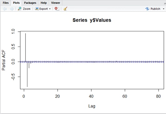
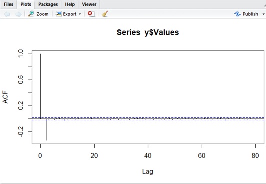
It’s hard to know the degree ( $p$ and $q$ ) of ARMA process, because it’s hard to distinguish whether it equals to $0$ or decreasing exponentially. (These are approximated values.) Then, in the real estimation process, the other criteria, such as AIC, BIC or Schwarz Information Criteria (SIC), is often used for finding the degree of time series. (Here I don’t describe about details, but please see my post for information criteria.)

Please see the following AR(2) and MA(2) examples for autocorrelation (ACF) and partial autocorrelation (PACF) in R. (The x-axis is lags, and the y-axis is correlation.)
You will find that these properties (ACF and PACF) obviously differ from models.

Sample code for AR(2) data generation and plotting

library(forecast)data_count <- 10000cons <- 70y1 <- 10phi1 <- 1.8phi2 <- -0.9e <- rnorm(data_count) * 10y2 <- cons + (phi1 * y1) + e[2]y <- data.frame(  Indexes=c(1, 2),  Values=c(y1, y2))for (i in 3:data_count) {  yi <- cons + (phi1 * y$Values[i-1]) + (phi2 * y$Values[i-2]) + e[i]  y <- rbind(y,data.frame(Indexes=c(i), Values=c(yi)))}# Autocorrelation plottingacf(  y$Values,  lag.max = 80,  type = c("correlation"),  plot = T)# Partial Autocorrelation plottingpacf(  y$Values,  lag.max = 80,  plot = T)

Autocorrelation plotting of AR(2)

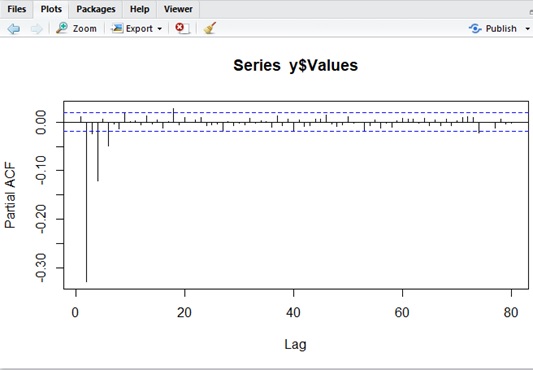
Partial Autocorrelation plotting of AR(2)

Sample code for MA(2) data generation and plotting

data_count <- 10000mu <- 70theta1 <- 1theta2 <- -1e <- rnorm(data_count) * 10y1 <- mu + e[1]y2 <- mu + e[2] + (theta1 * e[1])y <- data.frame(  Indexes=c(1, 2),  Values=c(y1, y2))for (i in 3:data_count) {  yi <- mu + e[i] + (theta1 * e[i-1]) + (theta2 * e[i-2])  y <- rbind(y,data.frame(Indexes=c(i), Values=c(yi)))}# Autocorrelation plottingacf(  y$Values,  lag.max = 80,  type = c("correlation"),  plot = T)# Partial Autocorrelation plottingpacf(  y$Values,  lag.max = 80,  plot = T)

Autocorrelation plotting of MA(2)

Partial Autocorrelation plotting of MA(2)

3. Estimate Parameters

Next we should estimate the parameters – $\phi_1,\phi_2,\cdots,\phi_p,\theta_1,\theta_2,\cdots,\theta_q$ and $\sigma$ in $\epsilon_t$ .
Once model is determined, you can use the standard estimation techniques to estimate parameters – such like, moment, least squares, or maximum likelihood.

For example, using the given data ${y_0, y_1, \cdots y_k}$ , you can analytically determine the parameter values ( $\phi_1,\phi_2,\cdots,\phi_p,\theta_1,\theta_2,\cdots,\theta_q, \sigma$ ) which maximize the likelihood of $\epsilon_t$ , in which I assume that $\epsilon_t$ is Gaussian distribution $\mathcal{N}(0, \sigma^2)$ .
Please see my post for maximum likelihood estimation (MLE). (In this post, I don’t explain details about MLE.)

After we have found model and parameters, we can survey the given data with the techniques of the statistical survey sampling.

Now, let me show you how you can estimate in programming with R.
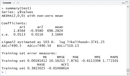
By using R or Python, you can estimate time series without any difficulties and quickly experiment with real data. You just use auto.arima() in forecast package in R.

The following is a brief R example, in which I have created the data of AR(2) ( $\phi_1 = 1.8,\phi_2 = -0.9$ ) and estimated with auto.arima() function.

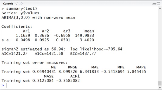
library(forecast)# create time-series data with ARMA(2, 0)data_count <- 1000cons <- 70y1 <- 10phi1 <- 1.8phi2 <- -0.9e <- rnorm(data_count) * 10y2 <- cons + (phi1 * y1) + e[2]y <- data.frame(  Indexes=c(1, 2),  Values=c(y1, y2))for (i in 3:data_count) {  yi <- cons + (phi1 * y$Values[i-1]) + (phi2 * y$Values[i-2]) + e[i]  y <- rbind(y,data.frame(Indexes=c(i), Values=c(yi)))}# analyzetest <- auto.arima(y$Values, seasonal = F)summary(test)

As you can see below, you can have a good result, $\phi_1 = 1.8564,\phi_2 = -0.9580$ .
(Note that the following ARIMA(p, 0, q) means ARMA(p, q).)

Let’s see another example.
The following data is generated by sin() with some noise. (This type of data will be easily analyzed with spectrum technique.) Let’s see how these cyclic data is represented by ARMA modeling.

library(forecast)data_count <- 200y <- data.frame(  Indexes=c(1:data_count),  Noise=rnorm(data_count))y$Values <-  150 + (100 * sin(pi * y$Indexes / 10)) + (5 * y$Noise)plot(x = y$Indexes, y = y$Values)test <- auto.arima(y$Values, seasonal = F)summary(test)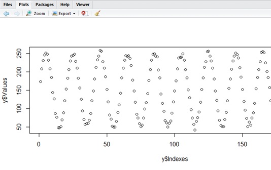

The following is the simulated plotting with result’s parameters in ARMA.
As you can see below, this model seems to be fitted closely to the cycle of given data.

library(forecast)data_count <- 200phi1 <- 1.1690phi2 <- 0.3636phi3 <- -0.6958c <- 149.9833 * abs(1 - phi1)e <- rnorm(data_count, sd = sqrt(66.94))y1 <- c + (phi1 * c) + e[1]y2 <- c + (phi1 * y1) + e[2]y3 <- c + (phi1 * y2) + (phi2 * y1) + e[3]y <- data.frame(  Indexes=c(1, 2, 3),  Values=c(y1, y2, y3))for (i in 4:data_count) {  yi <- c + (phi1 * y$Values[i-1]) + (phi2 * y$Values[i-2]) + (phi3 * y$Values[i-3]) + e[i]  y <- rbind(y,data.frame(Indexes=c(i), Values=c(yi)))}plot(y, type="l")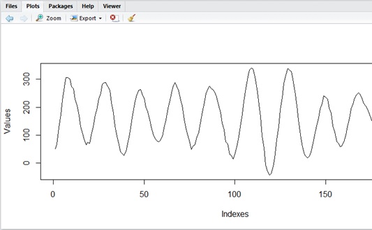

Note : You can simply use arima.sim() for simulation in R, but here I didn’t use this function for your understanding.

Now I have changed above data as follows. In this example, I have applied large white noise.

y <- data.frame(  Indexes=c(1:2000),  Noise=rnorm(2000))y$Values <-  20 + (10 * sin(y$Indexes / 30)) + (5 * y$Noise)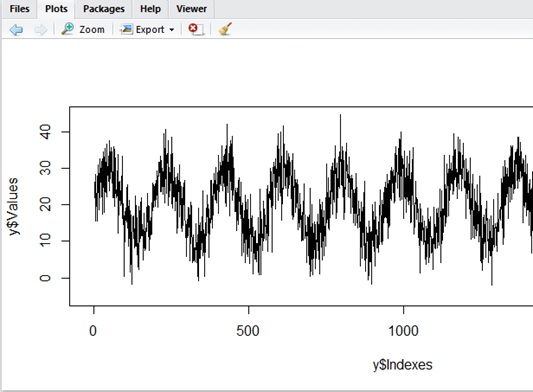

The following is the result by auto.arima() and simulated curve.
As you can see below, the estimation result is largely affected by the error noise of original data.

plot(x = y$Indexes, y = y$Values)test <- auto.arima(y$Values, seasonal = F)summary(test)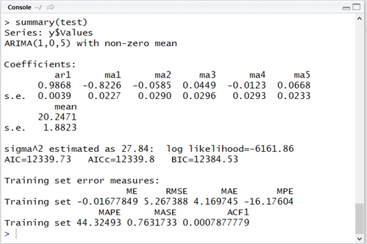

library(forecast)data_count <- 2000phi1 <- 0.9865theta1 <- -0.8565theta2 <- -0.0053theta3 <- 0.0187theta4 <- -0.0188theta5 <- 0.0864c <- 20.4084 * abs(1 - phi1)e <- rnorm(data_count, sd = sqrt(28.21))y1 <- c + (phi1 * c) + e[1]y2 <- c + (phi1 * y1) + e[2] + (theta1 * e[1])y3 <- c + (phi1 * y2) + e[3] + (theta1 * e[2]) + (theta2 * e[1])y4 <- c + (phi1 * y3) + e[4] + (theta1 * e[3]) + (theta2 * e[2]) + (theta3 * e[1])y5 <- c + (phi1 * y4) + e[5] + (theta1 * e[4]) + (theta2 * e[3]) + (theta3 * e[2]) + (theta4 * e[1])y <- data.frame(  Indexes=c(1, 2, 3, 4, 5),  Values=c(y1, y2, y3, y4, y5))for (i in 6:data_count) {  yi <- c + (phi1 * y$Values[i-1]) + e[i] + (theta1 * e[i-1]) + (theta2 * e[i-2]) + (theta3 * e[i-3]) + (theta4 * e[i-4]) + (theta5 * e[i-5])  y <- rbind(y,data.frame(Indexes=c(i), Values=c(yi)))}plot(y, type="l")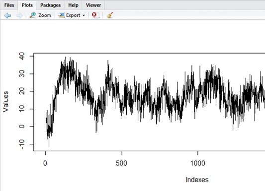

As this result shows us, the goal for estimation is to get the model of maximum possibility with explanatory variables, not to get the similar curve.
Once the result of $\epsilon_t$ (white noise) differs, the next result $y_{t+1}$ will also be changed by this difference. Without conditional expected value (which I’ll describe in the next section), these subsequent differences will cause the overall large difference between original data and estimated data, even though the estimated model is correct.

4. Forecasting ARMA Time Series

When the model and parameters are determined, now you can forecast the future values in time series with the generated model.
The forecasted values are called “conditional expected value” or “conditional mean”, because we should predict the future values $y_{k+1} , y_{k+2} , \cdots$ with $\epsilon_t$ distribution under the condition of given observed values (i.e, the values in the past) $\{y_0 , y_1 , \cdots , y_k \}$ . (I assume that $\epsilon_t$ represents Gaussian distribution.)

On contrary, the forecasting to show some range of possibility (e.g, the range of 95th percentile) is called “interval forecast”.
This possibility zone (mean squared errors, MSE) will get larger, when the time goes to the future.

For instance, the following is R example of this prediction (forecasting) in primitive AR(2) model.
In this curve :

The blue line is the conditional expected value.
The inner range (dark gray) is the interval forecast with the possibility of 85th percentile.
The outer range (light gray) is the interval forecast with the possibility of 95th percentile.

library("forecast")# create data with AR(2)data_count <- 1000cons <- 70y1 <- 10phi1 <- 1.8phi2 <- -0.9e <- rnorm(data_count) * 10y2 <- cons + (phi1 * y1) + e[2]y <- data.frame(  Indexes=c(1, 2),  Values=c(y1, y2))for (i in 3:data_count) {  yi <- cons + (phi1 * y$Values[i-1]) + (phi2 * y$Values[i-2]) + e[i]  y <- rbind(y,data.frame(Indexes=c(i), Values=c(yi)))}# estimate the modeltest <- auto.arima(y$Values, seasonal = F)summary(test)# plot with predictionpred <- forecast(  test,  level=c(0.85,0.95),  h=100)plot(pred)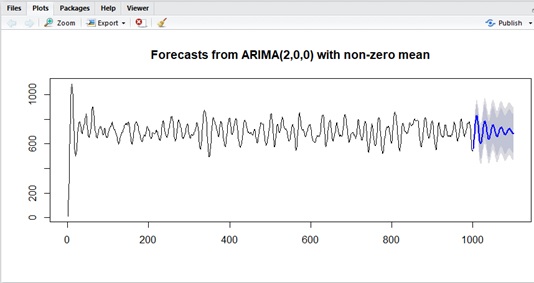

As you can see in the curve, the conditional expected value in AR converges to the expected value (the mean). And MSE converges to the variance of this model.
Therefore, it will be meaningless to forecast far future. (It will just be the mean value.)

In this post, I have discussed under the condition of stationarity.
In part 2, I will extend this idea to a non-stationary model and discuss more advanced topics about time series.

Categories: Uncategorized

Tagged as: MachineLearning

3 replies»

Erdogan Cevher says:
2018-03-21 at 03:41
arima.sim is a function of stats, not forecast package. “?arima.sim” in R console reveals this.
LikeLike
- Tsuyoshi Matsuzaki says:
  2018-03-22 at 10:25
  Thank you for your comment. I fixed my post.
  LikeLike
Dan Buckelew says:
2020-05-14 at 22:13
Can I just say what a relief to find somebody who really is aware of what theyre speaking about on the internet. You positively know methods to deliver a difficulty to mild and make it important. Extra folks have to read this and understand this side of the story. I cant believe youre not more common since you undoubtedly have the gift.
LikeLike

tsmatz

Professional Development, Data Science

Introduce Time Series Analysis with ARIMA (Part 1)

0. Before I start …

1. What is AR, MA, and ARMA

2. Find Model in Stationarity

3. Estimate Parameters

4. Forecasting ARMA Time Series

3 replies»

Leave a Reply Cancel reply

Recent Posts

Reinforcement Learning

Imitation Learning

Language Processing

Diffusion Models

Tags

Follow

Introduce Time Series Analysis with ARIMA (Part 1)

0. Before I start …

1. What is AR, MA, and ARMA

2. Find Model in Stationarity

3. Estimate Parameters

4. Forecasting ARMA Time Series

Share this:

Related

3 replies»

Leave a Reply Cancel reply

Recent Posts

Reinforcement Learning

Imitation Learning

Language Processing

Diffusion Models

Tags

Follow