Mathematical Introduction to Regression (and Related Topics)

By Tsuyoshi Matsuzaki on 2017-08-30• ( 1 Comment )

For the purpose of your beginning of machine learning, here I show you the fundamental mathematics behind regression with several examples.

Table of Contents

Introduction to Maximum Likelihood Estimation (MLE)
Interpretation of MLE into Information Theory
Regression Family (Logistic, Linear, Poisson, Gamma)
Link Functions
Evaluation Metrics
Other Methods for Regression (Further Learning …)

In this post, I’ll focus on parametric regression, which is a very basic method for regression.
There exist 2 main design choices for parametric regression as follows.

What surrogate loss should be used to measure the difference between actual distribution and estimated distribution ?
Which model is used to represent the distribution ?

For the former one, we apply (log) likelihood to measure the difference between actual distribution and estimated distribution. In the chapter 1 “Introduction to Maximum Likelihood Estimation”, I’ll explain the background math idea of this method. In the chapter 2 “Interpretation of MLE with Information Theory”, I’ll dig into MLE from a perspective of information theory.
For the latter part, I’ll explain a variety of models used today, in the chapter 3 “Regression Family”. The chapter 4 “Link Functions” will follow the other consideration for model designing.

There also exist other methods (such as, Bayesian inference, non-parametric methods, …) for solving practical problems. At the last part of this post (the chapter 6 “Other Methods for Regression”), I’ll introduce you the brief outline of these advanced methods

Mathematics behind ideas is very important to know exactly what the machine learning is. From this perspective, this post will explain mathematical ideas behind regression, but I’ll keep writing without difficult descriptions or complicated proofs.
I’ll also show you example code using R scripts, but even when you’re not familiar with R, it will be easy to understand, because I’ll keep my source code as simple as possible.
This post also gives you various insights in machine learning for the related topics.

1. Introduction to Maximum Likelihood Estimation (MLE)

One of primitive methods to find the optimal form of regression is to find parameters which maximizes the probability.
Maximum likelihood estimation (shortly, MLE) is based on this idea.

In this post, I’ll use several models (GLM regression family), each of which depends on specific problem respectively. But, regardless of the selected model, the following method (i.e, MLE) is commonly applied to solve regression problems through this post.

1. First, we should choose the appropriate statistical model (e.g, normal distribution, binomial distribution, Gamma distribution, etc) depending on each problem.

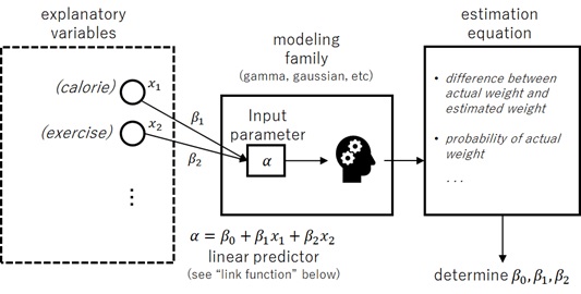
For instance, suppose, we want to predict human’s weight in some group, and we suppose that it depends on their daily calorie intake and daily amount of exercise.
In this case, we can apply linear regression model, because we can expect that the human weight will follow the normal distribution (Gaussian distribution).
In this example, the human’s weight is called a response variable (or label), and human’s daily calorie intake and daily amount of exercise are called explanatory variables (or features). Next I’ll give the expression of response variable using these explanatory variables.

2. The selected model (here, normal distribution) will have the corresponding parameters.
We suppose that these parameters of distribution depends on explanatory variables, and we then give the expression of these parameters using the formula of explanatory variables.

In above example, the Gaussian distribution (normal distribution) $\mathcal{N}(\mu, \sigma^2)$ has the parameter $\mu$ (the mean) and $\sigma$ (the standard deviation).
We now assume that $\mu$ (i.e, the human’s average weight) will depend on daily calorie intake $x_1$ and amount of exercise $x_2$ . We then suppose $\mu = \beta_0 + \beta_1 x_1 + \beta_2 x_2$ (the right-hand side is called linear predictor), where $\theta = \{ \beta_0$ , $\beta_1, \beta_2 \}$ are unknow parameters to be estimated.
Here I assume that $\sigma$ is a constant for any observation.

3. Finally we estimate $\beta_0$ , $\beta_1$ , and $\beta_2$ (unknown parameters in linear predictor) to fit to the observed actual data.

In above example, suppose, we have observed all human’s weights $y^{(0)}, y^{(1)}, \ldots, y^{(N-1)}$ , daily average of calorie intake $x_1^{(0)}, x_1^{(1)}, \ldots, x_1^{(N-1)}$ , and daily average of exercise $x_2^{(0)}, x_2^{(1)}, \ldots, x_2^{(N-1)}$ where $N$ is the number of observation.
For some fixed observation $(i)$ , we can then get the probability of $y^{(i)}$ when $x_1^{(i)}$ and $x_2^{(i)}$ is given, and we then denote this probability as $p_{\theta}(x_1^{(i)}, x_2^{(i)}, y^{(i)})$ . I note that this $p_{\theta}(x_1^{(i)}, x_2^{(i)}, y^{(i)})$ depends on $x_1^{(i)}$ , $x_2^{(i)}$ , $y^{(i)}$ , and parameters $\theta = \{ \beta_0$ , $\beta_1, \beta_2 \}$ . (Here we assume $\sigma$ is some constant.)
By multiplying all these probabilities by $p_{\theta}(x_1^{(0)}, x_2^{(0)}, y^{(0)}) p_{\theta}(x_1^{(1)}, x_2^{(1)}, y^{(1)}) \cdots p_{\theta}(x_1^{(N-1)}, x_2^{(N-1)}, y^{(N-1)})$ , we can now obtain a joint probability for all observed weights using unknown parameters $\theta = \{ \beta_0$ , $\beta_1, \beta_2 \}$ .
We can then estimate the optimal $\beta_0$ , $\beta_1$ , and $\beta_2$ to maximize this probability.

This method to maximize probability is called maximum likelihood estimation (MLE).

MLE is not the only thing to estimate the optimal parameters.
For instance, the ordinary least squares (OLS) is another estimation method to find parameters to minimize the difference between actual (observed) values $\{ y^{(i)} \}$ and the estimated values $\{ f_{\theta}(x^{(i)}) \}$ . This method finds parameter $\theta$ by the following quadratic loss function (or L2 loss function). :

$\displaystyle \arg \min_{\theta} \left\{ \sum_i (y^{(i)} - f_{\theta}(x^{(i)}))^2 \right\}$ .

Note : Or use mean squared error (shortly, MSE), which is the mean $\{ \sum_{i=0}^{N-1} (y^{(i)} - f_{\theta}(x^{(i)}))^2 \} / N$ , instead of the sum.

As I’ll show you later in this post, the solution to minimize a quadratic loss (or MSE) is equivalent to the solution to minimize likelihood (i.e, MLE) under Gaussian distribution. (For details, see linear regression in the following chapter 3.)

Note : Instead of a quadratic loss function, the following absolute loss function (or L1 loss function) can also be used to minimize the the difference between actual (observed) values and the estimated values. :
$\displaystyle \min_{\theta} \left\{ \sum_i | y^{(i)} - f_{\theta}(x^{(i)}) | \right\}$
It’s known that minimizing a quadratic loss gives the mean for training samples, while an absolute loss gives the median.

Sometimes MLE is ironically called “frequentist” approach, and you should remember that MLE is not always the best method for fitting in the given regression problems.
In the last part of this post, I’ll also discuss the shortcomings of MLE and show you other advanced alternatives.

2. Interpretation of MLE into Information Theory

There’s a close relation between the likelihood solution and the solution obtained from the principle of entropy.
Here I briefly show you how it’s related.

Note : You can skip this chapter, if you don’t have any interest to information theory behind methods.

Suppose, $p_{\theta}(x)$ is an estimated probability (which depends on parameters $\theta$ ) and $q(x)$ is an empirical probability (i.e, the probability of actual occurrence) for each occurrence $x$ .
In this assumption, the number of actual occurrence $x$ is $q(x) \cdot N$ (where $N$ is the number of observation), and the joint probability in MLE is then :

$\displaystyle P(\theta) = \prod_x p_{\theta}(x)^{q(x) \cdot N}$

Maximizing $P(\theta)$ is equivalent to minimizing the following equation. :

$\displaystyle -\frac{1}{N} \log P(\theta) = - \sum_x q(x) \log p_{\theta}(x)$

This formula $H(q, p) = - \sum_x q(x) \log p(x)$ is called a cross-entropy loss function (or log loss function).
This shows that minimizing cross-entropy loss is equivalent to maximizing the log likelihood.

Note : In neural networks, a cross-entropy function is often used as a loss function to quantify the difference between true values and estimated values. (The loss should then be minimized to optimize neural networks.)

According to information theory, the following $H(p)$ is known as entropy and it’s known to be a quantity of information to represent distribution $p$ . :

$\displaystyle H(p) = - \int p(x) \log p(x) dx$

And the following $KL(p || q)$ is known as KL divergence (Kullback-Leibler divergence) or relative entropy. :

$\displaystyle KL(p || q) = - \int p(x) \log \frac{q(x)}{p(x)} dx$

In information theory, it’s known that the stable probability distribution (i.e, randomness) leads to large entropy and you can then find optimal distribution by finding distribution to maximize entropy (which is called maximum entropy principle).
For instance, the continuous distribution to maximize entropy is known to be Gaussian distribution. A lot of possibilities in natural state can be written by exponential formula – a set of which distributions are called exponential family (see this Wikipedia) -, and these distributions also have maximum entropy in some constraints.

On contrary, KL divergence (or relative entropy) is often used as a distance of distributions between $p$ and $q$ , in which KL divergence always satisfies $KL(p||q) \geq 0$ with equality if, and only if, $p(x) = q(x)$ .

As you can easily see, maximizing entropy $H(p)$ is equivalent to minimizing KL divergence $KL(p||q)$ under the assumption that $q$ is an uniform distribution (i.e, uniformly distributed in discrete space).

Note : For these background behind information theory, see chapter 1.6 in “Pattern Recognition and Machine Learning” (Christopher M. Bishop, Microsoft).

As you can also see, $H(q, p) = H(q) + KL(q || p)$ . The maximum likelihood on exponential family, hence, is also a solution to minimize KL divergence between estimated distribution and empirical distribution. (I note that $KL(q || p) \neq KL(p || q)$ .)
Here I don’t go into details, but it’s also known that maximum likelihood on exponential family is a dual problem of maximizing entropy, subject to expectation constraints. (This principle is applied in some specific machine learning tasks – such as, Inverse Reinforcement Learning, etc.)

3. Regression Family

In machine learning, different statistical model is used to address each problem respectively.
In this section, I’ll pick up several popular models used in regression, and show you how MLE is applied.
(This section will be the main part of this post.)

Note : All statistical models discussed in this post belongs to exponential family. (See above.)
In this chapter, I’ll separate topics into each models, but all the theory written in this post can be generalized as the theory of exponential family.
Later (in the chapter 6) I’ll briefly discuss how to solve more difficult formula which doesn’t belong to exponential family – such as, Gaussian Mixture Models (GMM), etc.

Logistic Regression

Binomial regression with logit link function is called logistic regression. (Later I’ll show you what “logit link function” means.)
Now let’s briefly see the logistic regression example.

Suppose, it has the probability $p \; (0 \leq p \leq 1)$ of success occurrence for each trials (experiments). We try $N$ independent experiments and the count of success is $y_1$ times. i.e, it fails $y_2 = N - y_1$ times.
In this assumption, it’s known that the probability of this occurrence is :

$\displaystyle P(y_1, y_2) = {}_{y_1 + y_2}C_{y_1} p^{y_1} (1-p)^{y_2}$

where $\displaystyle {}_{a}C_{b} \stackrel{\mathrm{def}}{=} \frac{a(a - 1)(a - 2) \cdots (a - (b - 1))}{b !}$

This probability space is called binomial distribution.

When $y_1$ and $y_2$ are given, this equation will then be denoted as follows by using only unknown parameter $p$ .

$P(p) = {}_{y_1 + y_2}C_{y_1} p^{y_1} (1-p)^{y_2}$

When a lot of pairs $\{ (y_1^{(0)}, y_2^{(0)}), (y_1^{(1)}, y_2^{(1)}), \ldots \}$ are given, the joint probability will then be given by the multiplication as follows. (Because each occurrence is independent.)

$\displaystyle \prod_{i} {}_{y_1^{(i)} + y_2^{(i)}}C_{y_1^{(i)}} p^{y_1^{(i)}} (1-p)^{y_2^{(i)}}$

Now let’s consider using an example. :
Suppose, we have fishes in the fish tank, and we survey the survival rate depending on the amount of given food and the amount of given oxygen as follows.

Alive(y1) Dead(y2) Food(x1) Oxygen(x2)39 11 300 200030 20 150 120012 38 100 1000...

Now we denote the probability of survival in i-th case as $p^{(i)}$ . And I assume that it depends on the food $x_1^{(i)}$ and oxygen $x_2^{(i)}$ , such as : $p^{(i)} = \beta_0 + \beta_1 x_1^{(i)} + \beta_2 x_2^{(i)}$ . (The right-hand side of this equation is the linear predictor.)

The joint probability is then written as follows. (Suppose, all pairs $(x_1^{(i)},x_2^{(i)},y_1^{(i)},y_2^{(i)})_{i=0,1,\ldots}$ are given values.)

$\displaystyle P(\beta_0, \beta_1, \beta_2) = \prod_{i} {}_{y_1^{(i)} + y_2^{(i)}}C_{y_1^{(i)}} (\beta_0 + \beta_1 x_1^{(i)} + \beta_2 x_2^{(i)})^{y_1^{(i)}} (1- (\beta_0 + \beta_1 x_1^{(i)} + \beta_2 x_2^{(i)}))^{y_2^{(i)}}$

Our goal is to find the optimal parameters $\beta_0$ , $\beta_1$ , $\beta_2$ to maximize the joint probability $P$ .
The solution is then analytically obtained by the gradient descent or Newton-Raphson method with partial derivatives. (In this post, I’ll skip the detailed procedure for these methods.)

In this assumption, there exists a trick. Is that really $p^{(i)} = \beta_0 + \beta_1 x_1^{(i)} + \beta_2 x_2^{(i)}$ ?
In logistic regression, the following formula is often used for the linear predictor, instead of $p^{(i)} = \beta_0 + \beta_1 x_1^{(i)} + \beta_2 x_2^{(i)}$ .
This formula is called sigmoid function.

$\displaystyle p^{(i)} = sigmoid(\beta_0 + \beta_1 x_1^{(i)} + \beta_2 x_2^{(i)}) \stackrel{\mathrm{def}}{=} \frac{1}{1+exp(-(\beta_0 + \beta_1 x_1^{(i)} + \beta_2 x_2^{(i)}))}$

In the later section (in the chapter 4), I’ll give you the reason why this formula is used. (So, please skip the detailed reason here.)

As a result, the estimation function of the logistic regression will then be re-written as follows :

$\displaystyle P(\beta_0, \beta_1, \beta_2)=\prod_{i} {}_{y_1^{(i)} + y_2^{(i)}}C_{y_1^{(i)}} sigmoid(\beta_0+\beta_1 x_1^{(i)} + \beta_2 x_2^{(i)})^{y_1^{(i)}} (1-sigmoid(\beta_0+\beta_1 x_1^{(i)}+\beta_2 x_2^{(i)}))^{y_2^{(i)}}$

Note : It’s known that it’s possible to analytically find the optimal $\beta_0, \beta_1, \beta_2$ when it’s exponential family.

Now let’s see the program code with R script.
First I have generated sample data (1000 rows) with $\beta_0 = -15$ , $\beta_1 = 4$ , $\beta_2 = 2$ and random noise (rbinom() function).

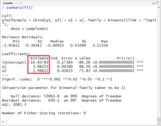
library(e1071) # for sigmoid func###### create sample data with rbinom###### y1 : number of alive# y2 : number of dead# x1 : food# x2 : oxygen#####n_sample <- 1000total <- 50b0 <- -15b1 <- 4b2 <- 2x1 <- runif(  n = n_sample,  min = 0,  max = 5)x2 <- runif(  n = n_sample,  min = 0,  max = 5)probs <- sigmoid(b0 + b1 * x1 + b2 * x2)y1 <- rbinom(  n = n_sample,  size = total,  prob = probs)y2 <- total - y1sampledat <- data.frame(  x1 = x1,  x2 = x2,  y1 = y1,  y2 = y2)

To estimate the optimal parameters, call glm() function in R script as follows.

With binomial() setting, this function solves regression problem by binomial distribution.
By “link=logit” setting, a logistic sigmoid function (see above) is used in a linear predictor.

###### Estimate#####fit <- glm(  cbind(y1, y2) ~ x1 + x2,  data = sampledat,  family = binomial(link = "logit"))summary(fit)

Note : The default link function of binomial distribution is “logit” in R. You don’t then need to specify link = "logit" explicitly. (Here I have explicitly specified for your understanding.)

By running this code, we can get the optimal result : $\beta_0 = -14.95783$ , $\beta_1 = 3.98255$ and $\beta_2 = 1.99622$ . (See the following output.)
As you saw above, this result is near the actual values.

Let’s see another example.
The following dataset is similar to the previous one (sampledat), but each of rows has $t$ flag (“survival” column in below) which identifies “Dead” as 0 and “Alive” as 1, instead of previous $y_1$ (count of aliveness) and $y_2$ (count of death).

sampledatA

Survival(t) Food(x1) Oxygen(x2)1 300 20000 100 10001 300 20000 100 10000 300 20001 300 20001 100 1000...

Now I denote $t$ in i-th trial as $t^{(i)} \in \{0,1\}$ . The joint probability will then be given as follows. (The definition of $p^{(i)}$ is the same as above.)
Same as above, we can get the optimal parameters by solving the maximum likelihood of this joint possibility.

$\displaystyle P(\beta_0,\beta_1,\beta_2) = \prod_{i} {p^{(i)}}^{t^{(i)}} (1-p^{(i)})^{1-t^{(i)}}$

In order to get this estimated results ( $\beta_0$ , $\beta_1$ , and $\beta_2$ ), you can just run the following R script.

## with "Survival" column t (0 or 1)fit2 <- glm(  t ~ x1 + x2,  data = sampledatA,  family = binomial(link = "logit"))summary(fit2)

As you can see, this dataset (above sampledatA) can also be written by the following format (sampledatB), which is the same format as previous one.
Of course, this then leads to the same solution, $\beta_0$ , $\beta_1$ , and $\beta_2$ .

sampledatB

Alive(y1) Dead(y2) Food(x1) Oxygen(x2)3 1 300 20001 2 100 1000...

Poisson Regression

Let’s see another example in regression family.

Suppose, some event occurs $\lambda$ times in some time-interval.
It’s known that the probability $P$ of $k$ times occurrence of the same event in the same interval is then written as follows.
This stochastic distribution is called Poisson distribution.

$\displaystyle P(k | \lambda) = \mathrm{e}^{-\lambda} \frac{\lambda^k}{k!}$

Now let’s consider using a following example. :
Here we plant some seeds in our garden, and we survey how many seeds germinate depending on the amount of water and fertilizer.
In this model, we consider that $\lambda$ (the average of germinating seeds) depends on the water $x_1$ and fertilizer $x_2$ . We might think that the parameter $\lambda$ will have the following relation.

$\displaystyle \lambda = \beta_0 + \beta_1 x_1 + \beta_2 x_2$

In practical use-case in Poisson regression, the following function is often used as $\lambda$ , instead of the previous representation. (The inverse of this function (i.e, $\log{\lambda}$ ) is called the log link function.)
In the later section, I’ll also give you the reason why this link function is used. (Please ignore here for this formula of link function.)

$\displaystyle \lambda = \mathrm{e}^{\beta_0 + \beta_1 x_1 + \beta_2 x_2}$

Suppose, a lot of data of $k$ , $x_1$ and $x_2$ are given as follows.

Germinating(k) Water(x1) Fertilizer(x2)11 300 20008 150 12005 100 1000...

We can then define the joint probability by multiplication as follows.
Our goal is to find the parameters $\beta_0$ , $\beta_1$ , $\beta_2$ which maximize the following possibility $P$ by the maximum likelihood estimation.

$\displaystyle P(\beta_0, \beta_1, \beta_2) = \prod_{i} \exp(-\exp(\beta_0 + \beta_1 x_1^{(i)} + \beta_2 x_2^{(i)})) \frac{\exp(\beta_0 + \beta_1 x_1^{(i)} + \beta_2 x_2^{(i)})^{k^{(i)}}}{k^{(i)}!}$

Note : In most cases, the estimation is performed by minimizing $-log P = -log(\prod_{i} P^{(i)}) = -\sum_{i} log P^{(i)}$ , instead of maximizing $P$ .
See about loss function in above note.

Let’s see the following simple example with R to solve this regression problem.
Using rpois() function, here we also generate the simulated data (1000 rows) with random noise (errors) using $\beta_0 = 0.2$ , $\beta_1 = 0.5$ , $\beta_2 = 0.4$ . And I then estimate parameters with glm() function.

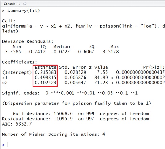
###### create sample data with rpois###### y : germinating# x1 : water# x2 : fertilizer#####n_sample <- 1000b0 <- 0.2b1 <- 0.5b2 <- 0.4x1 <- runif(  n = n_sample,  min = 0,  max = 5)x2 <- runif(  n = n_sample,  min = 0,  max = 5)lamdas <- exp(b0 + b1 * x1 + b2 * x2)y <- rpois(  n = n_sample,  lambda = lamdas)sampledat <- data.frame(  x1 = x1,  x2 = x2,  y = y)###### Estimate#####fit <- glm(  y ~ x1 + x2,  data = sampledat,  family = poisson(link = "log"))summary(fit)

Note : The default link function of Poisson distribution is “log” and then you do not need to specify link = "log" explicitly in R.

As you can see in the following output, the estimated results are $\beta_0 = 0.215383$ , $\beta_1 = 0.498815$ and $\beta_2 = 0.402523$ .
As you can find, the result is well estimated.

Linear Regression (Gaussian Regression)

Linear regression (Gaussian regression) will be mostly primitive and widely used regression model in machine learning, but you should understand how it’s related to the familiar Gaussian distribution (normal distribution).

First, we consider this regression very straightforward to ease the problems.
Suppose, the formula with primitive linear expression is given. Now we want to find the optimal parameters $\beta_0, \beta_1, \ldots$ to fit to the observed data.

$\displaystyle y = \beta_0 + \beta_1 x_1 + \beta_2 x_2 + \cdots$

As you saw above in previous examples, we have applied maximum likelihood estimation (MLE), which will maximize the joint possibility in stochastic distribution models.
But here, we don’t use MLE and dare to use the ordinary least squares (OLS) for estimation, which minimize the sum of distance squares (or MSE) between observed values and predicted values.
Now let’s see the brief example.

For simplicity, we assume that the only $x_1$ is used for explanatory variable, i.e, $y = f(x_1) = \beta_0 + \beta_1 x_1$ .
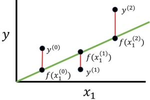
In ordinary least squares (OLS) method, first we calculate each distance between the observed value $y^{(i)}$ and predicted value $f(x_1^{(i)})$ . (See below.)

The value of distance might be positive or negative. We then sum up the square of each distance as follows.
Our goal is to find the optimal parameters $\beta_0$ , $\beta_1$ to minimize the following $E$ (where $y^{(0)}$ , $y^{(1)}$ , $y^{(2)}$ , … are observed values).

$\displaystyle E = (y^{(0)} - f(x_1^{(0)}))^2 + (y^{(1)} - f(x_1^{(1)}))^2 + (y^{(2)} - f(x_1^{(2)}))^2 + \cdots$

Why is it called “Gaussian” ?
Now let’s consider the normal distribution (Gaussian distribution) $\mathcal{N}(\mu, \sigma^2)$ . Suppose the standard deviation $\sigma$ (the square root of variance) is a constant value for any observation and the probability depends only on parameter $\mu$ (the mean).
We then consider the maximum likelihood estimation (MLE) for this Gaussian distribution.

Suppose $\mu^{(i)} = \beta_0 + \beta_1 x_1^{(i)}\;\;(i=0,1,\ldots)$ , and introduce a small range $[y^{(i)} - \Delta,y^{(i)} + \Delta]$ (where $\Delta$ is some fixed small value) instead of $y^{(i)}$ . (Because $y^{(i)}$ is the value of probability density, not probability.)
If $\Delta$ is very small, the joint probability would then be written as follows. :

$\displaystyle P(\beta_0, \beta_1) = \prod_{i} \frac{2 \Delta}{\sqrt{2 \pi \sigma^2}} exp(-\frac{(y^{(i)}-\beta_0-\beta_1 x_1^{(i)})^2}{2 \sigma^2})$

Now we apply the logarithm for this equation (i.e, log-likelihood) and it’s then written by :

$\displaystyle \log{P(\beta_0, \beta_1)} = \sum_{i} \left\{log(2\Delta) - \frac{1}{2}\log(2\pi\sigma^2) - \frac{(y^{(i)}-\beta_0-\beta_1 x_1^{(i)})^2}{2 \sigma^2}\right\}$

As you can easily see, we can get the maximum likelihood when we minimize $\displaystyle \sum_{i} (y^{(i)}-\beta_0-\beta_1 x_1^{(i)})^2$ . (Because $log(2\Delta)$ and $\frac{1}{2}\log(2\pi\sigma^2)$ doesn’t depend on $\beta_0$ and $\beta_1$ .)
Therefore, maximum likelihood estimation (MLE) under Gaussian distribution (i.e, linear regression) is equivalent to applying ordinary least squares (OLS) method (minimizing MSE).

Note : When the standard deviation (or variance) is unknown and the number of observations is small, we sometimes consider the marginal distribution of Gaussian distribution on the precision (which is the inverse of a variance), instead of using Gaussian distribution. This distribution is called Student’s t-distribution.
It’s known that Student’s t-distribution is more robust to outliers than Gaussian distribution. (Gaussian distribution is a special case of Student’s t-distribution.)

It’s known that various phenomenon in nature (including random trials) will follow Gaussian distribution, because the continuous (not discrete) distribution to maximize an entropy is Gaussian distribution. (See above note for entropy in information theory.)
Therefore linear regression is then applied in a lot of cases in practices.

Suppose, the average amount of human’s daily salt intake might also follow Gaussian distribution $\mathcal{N}(\mu, \sigma^2)$ , with mean $\mu$ and standard deviation $\sigma$ . (The curve of population will have a peak in the most popular value $\mu$ and will also be symmetric.)
Also, suppose, the mean $\mu$ of salt intake relies on one’s weight $x_1$ and it has the linear relation.
In this case, you can get the regression result by MLE under Gaussian distribution (or OLS) with linear predictor $y = \beta_0 + \beta_1 x_1$ .

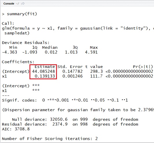
Let’s see the following simple example with R script.
As you can see below, here I generate the data (1000 rows) with random noise (errors) using $\beta_0 = 44$ , $\beta_1 = 0.14$ and rnorm() function. (The data will then be generated on normal distribution.)
And I then estimate parameters with glm() function.

###### create sample data###### y : salt intake (g / 10 days)# x1 : weight (pond)#####n_sample <- 1000b0 <- 44b1 <- 0.14x1 <- runif(  n = n_sample,  min = 45,  max = 180)epsilon <- rnorm(  n = n_sample,  mean = 0,  sd = 1.57)  # noise (variance)y <- b0 + b1 * x1 + epsilonsampledat <- data.frame(  x1 = x1,  y = y)###### Estimate#####fit <- glm(  y ~ x1,  data = sampledat,  family = gaussian(link = "identity"))summary(fit)

Note : link="identity" means the link function with $y = x$ . (That is, the linear predictor is not modified to other formula.)
The default link function of Gaussian distribution is “identity” in R. Then you do not need to specify link = "identity" explicitly.

As you can see in the output, the estimated results are $\beta_0 = 44.085248$ and $\beta_1 = 0.139133$ . (It’s well-estimated.)

Gamma Regression

Finally I’ll introduce Gamma regression.

Suppose, some event occurs $r$ times in the unit (i.e, 1) interval.
It’s known that the probability density function $p$ of $s$ times’ occurrence in the interval $y$ becomes as follows :

$\displaystyle p(y | s, r) = \frac{r^s}{\Gamma(s)} y^{s-1} exp(-ry)$

where $\Gamma()$ is Gamma function.

Note : Same as Gaussian distribution, it’s a probability density function, not a probability function.
Same as MLE in linear regression, you should use integral or get the probability with some fixed small range $\Delta$ .

Here I don’t go details about this function’s form, but Gamma function is an extended form of factorial operation $\Gamma(n+1) = n!$ (where $n$ is positive integer) for real or complex numbers. (See “Wikipedia : Gamma function” for details.)

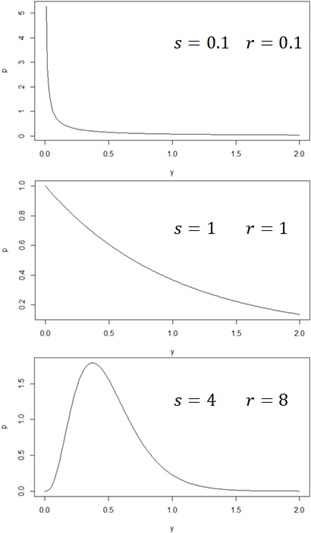
Note : I show you examples of Gamma distribution for several $s$ and $r$ pairs as follows.

This regression is often used for the analytics, such as, waiting time, time between failure, accident rate, so on and so forth.
There exist two parameters $s$ , $r$ – called “shape” and “rate” respectively, but we suppose $s$ is always the same (i.e, constant) for any observation in this regression.

For example, let’s consider the time of the failure (breakdown) for some equipment using Gamma regression.
Suppose, this occurrence depends on the count of initial bugs $x_1$ and the number of claims by customers $x_2$ . Also suppose, 1 failure (breakdown) is caused by approximately 10 times errors, i.e, $s = 10$ .
When the count of initial bugs increases, the errors in production would also increase. That is, when $x_1$ (the count of initial bugs) increases, $r$ (the count of errors for unit interval) will then increase, though $s\;(=10)$ (the count of errors for failure) is always a constant. On the contrary, the average $\frac{s}{r}$ decreases.

In the practical use-case, the following inverse link function is then often used for Gamma regression. (I’ll describe the details about this link function later.)
Here $\frac{1}{r}$ is called “scale”.

$\displaystyle \frac{1}{r} \propto \frac{s}{r} = \frac{1}{\beta_0 + \beta_1 x_1 + \beta_2 x_2}$

Note : Here I don’t explain about details, but $s$ (shape) can also be estimated by mathematical steps. (Because it’s known that the variance $\sigma^2$ of Gamma distribution is $\frac{s}{r^2}$ .)

Let’s see the following simple example with R script.
As you can see below, here I generate the simulated data with random noise (errors) using $\beta_0 = 0.5$ , $\beta_1 = 0.02$ , $\beta_2 = 0.01$ and rgamma() function.
And I then estimate parameters with glm() function.

###### create sample data with rgamma###### y : time to failure# x1 : number of initial bugs# x2 : number of customer claims#####n_sample <- 1000shape <- 10b0 <- 0.5b1 <- 0.02b2 <- 0.01x1 <- runif(  n = n_sample,  min = 1,  max = 5)x2 <- runif(  n = n_sample,  min = 11,  max = 15)rate <- (b0 + b1 * x1 + b2 * x2) * shapey <- rgamma(  n = n_sample,  shape = shape,  rate = rate)sampledat <- data.frame(  x1 = x1,  x2 = x2,  y = y)###### Estimate#####fit <- glm(  y ~ x1 + x2,  data = sampledat,  family = Gamma(link = "inverse"))summary(fit)

As you can see in the following output, the estimated results are $\beta_0 = 0.504847$ , $\beta_1 = 0.021330$ and $\beta_2 = 0.008929$ . (It’s well-estimated.)

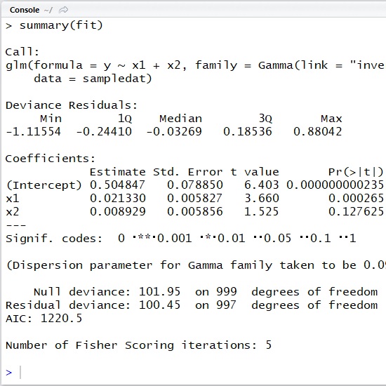
If you need the value of shape ( $s$ ), you can use the following gamma.shape() in MASS package. (You can then get the original model of Gamma distribution.)

library(MASS)...# you can get shape as follows.test <- gamma.shape(fit, verbose = TRUE)

4. Link Functions

In the previous examples, I have used several link functions without making it clear, but now it’s time to explain about link functions.

Designing link functions is also important part in regression modeling.

Note : The inverse of link function is called activation function. In this section, I’ll discuss using a formula of activation functions .

Log Link Function

Remind the previous Poisson regression example (example of plant’s germination).

I assume that $\lambda$ (i.e, the average of germinating) has the following linear predictor :

$\lambda = \beta_0 + \beta_1 x_1 + \beta_2 x_2 \;\;\; (1)$

Suppose, the seeds have germinated 1.5 times a lot by some increase of water. And also the seeds have germinated 1.2 times a lot by some increase of fertilizer.
If you increase the same amount of both water and fertilizer, the seeds would germinate 1.5 + 1.2 = 2.7 times a lot ?
Of course, Not. We will expect that it will germinate 1.5 * 1.2 = 1.8 times a lot.

Therefore formula (1) doesn’t represent our expected model.
Now we correct this formula as follows.

$\displaystyle \lambda = \mathrm{e}^{\beta_0 + \beta_1 x_1 + \beta_2 x_2}$

This is called a log link function. The reason of this name is that the linear predictor $\beta_0 + \beta_1 x_1 + \beta_2 x_2$ equals to $\log{\lambda}$ .

When we replace with $\beta^{\prime}_0 = \mathrm{e}^{\beta_0}$ , $\beta^{\prime}_1 = \mathrm{e}^{\beta_1}$ , $\beta^{\prime}_2 = \mathrm{e}^{\beta_2}$ , we then get the following formula (2).

$\displaystyle \lambda = \beta^{\prime}_0 {\beta^{\prime}_1}^{x_1} {\beta^{\prime}_2}^{x_2} \;\;\; (2)$

When ${\beta^{\prime}_1}^{x_1} = 1.5$ and ${\beta^{\prime}_2}^{x_2} = 1.2$ , the total effects would be ${\beta^{\prime}_1}^{x_1} \cdot {\beta^{\prime}_2}^{x_2} = 1.8$ times.
Using formula (1), it can also be a negative number when $x_1$ or $x_2$ decreases. But, with formula (2), it won’t happen.
For these reasons, log link function is often used in the regression under Poisson distribution.

Of course, the log link function would not always be the answer in Poisson regression. The important thing is to understand this background idea and use the appropriate link function along with your problems.

Logit Link Function

The logit link function is used for representing the value between 0 and 1. Therefore it’s then often used in logistic regression. (This idea is also used in 2-class classification task in today’s neural networks.)
Let’s go dive into logit link function.

Remind the previous logistic regression example (the fish survival example).
Now we consider the following logical model. :

Each input of $x_1$ (food) and $x_2$ (oxygen) is having the weight $w_1$ and $w_2$ respectively.
For instance, when the oxygen is so critical rather than the food for survival, $w_2$ will become larger than $w_1$ .
It then gets the total weight by $\sum_{i} w_i x_i = w_1 x_1 + w_2 x_2$ .
Compare this total weight with some fixed threshold $b$ .
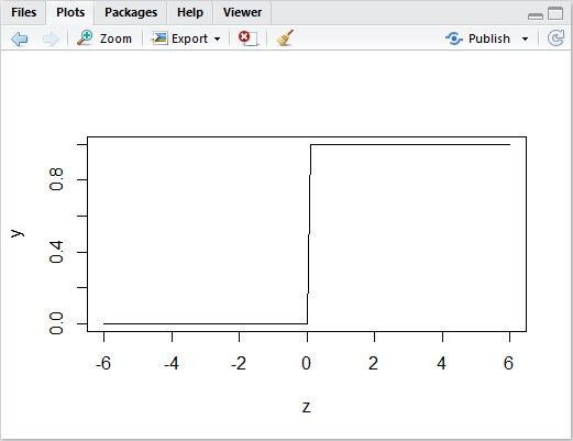
If it’s exceed $b$ , the result $y$ becomes $1$ . Otherwise, the result $y$ becomes $0$ . (See the following picture.)

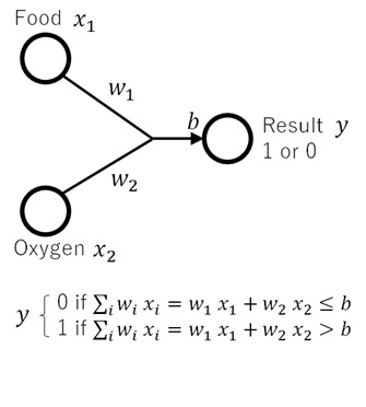
This model represents the aspect of the actual decision mechanism. But one important drawback is that it is not continuous and it’s a discrete function.
The following picture shows the plotting when we suppose $z = \sum_{i} w_i x_i - b$ .
Because of this, some mathematical operations (such as, differentiation) will be difficult to apply.

Therefore we introduce the following activation function called a logistic sigmoid function.

$\displaystyle sigmoid(z)$
$\displaystyle = \frac{1}{1 + \mathrm{e}^{-z}}$
$\displaystyle = \frac{1}{1 + \exp(-\sum_{i} w_i x_i + b)}$

As you can see below, the curve of this sigmoid is very similar to the previous one, but it’s continuous (not discrete).

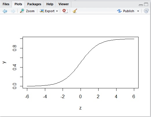
Note : For simplicity, here I discuss things on the assumption that the formula of logistic sigmoid function is given. However, this formula can be derived statistically.
Please remind that the formula of Gaussian distribution (normal distribution) has exponential part, and you will then find the logistic sigmoid function is well-defined for the inputs with Gaussian distribution. Not only Gaussian distribution, but other well-known distributions in exponential family are all statistically related to logistic sigmoid function (when it’s in 2 classes) and softmax function (when it’s in multiple classes).
I also note that there is close similarity between logistic sigmoid function and the cumulative distribution of Gaussian distribution. The cumulative of Gaussian distribution is sometimes approximated by using a logistic sigmoid function.

Now we suppose $w_2 = \beta_2$ , $w_1 = \beta_1$ , $-b = \beta_0$ , and we can then get the probability $p$ (i.e, probability of alive) as follows.

$\displaystyle p = \frac{1}{1 + \exp(-(\beta_0 + \beta_1 x_1 + \beta_2 x_2))}$

The logit link function is the inverse of this logistic sigmoid function as follows. :

$\displaystyle \beta_0 + \beta_1 x_1 + \beta_2 x_2 = sigmoid^{-1} (p) = \log{\frac{p}{1-p}}$

Note : As you can see, this $1 - p$ is representing the probability of dead. This ratio of $\frac{p}{1 - p}$ is then called odds.

In neural networks, this idea (sigmoid) is extended, such as :

As you saw above, sigmoid() is in the range (0, 1). Now you can consider tanh() as the analog of sigmoid for the range (-1, 1).
Since $tanh(z) = 2 sigmoid(2z)-1$ , then tanh() is equivalent to sigmoid() except for the range.
As you saw above, the input (which might positively exceed 1 and also negatively exceed -1) is interpreted into 2 classes (i.e, 0 or 1), by a logistic sigmoid function. For the multiple $N$ classes ( $N \geq 2$ ), you can use softmax function instead, in which the possibility for class $m$ is represented by
$e^{z_m}/(e^{z_1} + e^{z_2} + \cdots + e^{z_N})$
where $z_i$ indicates the linear predictor’s output (sometimes, called “logits”) for class $i$ .
Since $e^{z_1}/(e^{z_1} + e^{z_2}) = 1/(1+e^{-(z_1-z_2)})$ , then you will find that it’s the extension of the logistic sigmoid function for multiple classes.

Note : In softmax function, the output $z_i$ is called logits.
The logits will be any real number, but $e^{z_i}$ will become positive number, and finally it’s normalized (into the range (0, 1)) by $e^{z_i}/(e^{z_1} + e^{z_2} + \cdots + e^{z_N})$ .
The softmax function is often used for activation function in today’s neural networks.
Note : In neural networks, it sometimes introduces the following parameter $T$ , called temperature. When $T \ll 1$ , the distribution becomes peaked around the origin. On the other hand, when $T \gg 1$ , the distribution flattens out.
There’s a trade-off between coherence (low temperature) and diversity (high temperature).
$e^{(z_m/T)}/(e^{(z_1/T)} + e^{(z_2/T)} + \cdots + e^{(z_N/T)})$

Inverse Link Function

$\frac{1}{p}$ is called the inverse link function, where $p$ is the predicted parameter.

Remind the previous Gamma regression example (example of errors and failure).
In this example, predicted parameter $p$ is the scale parameter $\frac{s}{r}$ (where $s$ (constant) is shape and $r$ is rate).

Because $\frac{1}{p} = \frac{r}{s}$ , then it can also be denoted as follows using $\beta^{\prime}_0, \beta^{\prime}_1, \beta^{\prime}_2$ . :

$r = \beta^{\prime}_0 + \beta^{\prime}_1 x_1 + \beta^{\prime}_2 x_2$
where $\beta^{\prime}_0=\beta_0 s$ , $\beta^{\prime}_1=\beta_1 s$ , $\beta^{\prime}_2=\beta_2 s$

As I have explained in Gamma regression, $r$ (rate) means “the occurrence count in the unit (1) interval”. Then $\frac{1}{r}$ means “the average interval between occurrence”. This $\frac{1}{r}$ is called “scale”.
In case when the linear predictor is proportional to the scale (i.e, inversely proportional to the rate), you should specify identity link function in Gamma regression as follows, instead of specifying inverse link function.

fit <- glm(  y ~ x1 + x2,  data = sampledat,  family = Gamma(link = "identity"))

Note (About Offset) :
When you want to specify some input variable without predicted coefficient, such as $\beta_0 + \beta_1 x_1 + \beta_2 x_2 + {\bf x_3}$ , you can use offset.
For instance, now we introduce new input variable “observation count” ( ${\bf x_3}$ ) in the previous example of Poisson regression (example of plant’s germination).
Then the following linear predictor will be used.
$\displaystyle {\bf x_3} exp(\beta_0 + \beta_1 x_1 + \beta_2 x_2) = \exp(\beta_0 + \beta_1 x_1 + \beta_2 x_2 + \log{\bf x_3})$
In such a case, you can use offset as follows.
fit <- glm(  y ~ x1 + x2,  data = sampledat,  family = poisson(link = "log"),  offset = log(x3))
You might think that you could just divide the result $y$ by ${\bf x_3}$ in this case, instead of using offset. However, by using offset, you can run regression without changing the variance or other mathematical attributes.

5. Evaluation Metrics

After the model is trained, you should evaluate how well it fits to the actual data.

Here I’ll only show you the popular evaluation metrics for regression, with its notations.
By using these metrics, you can quantitatively measure how well the model fits.

The good model will fit not only to given data (the data used in training), but also to unseen data. For this reason, the unseen data (which is not used in training) is usually used for the evaluation.

Mean Squared Error (MSE)

$\displaystyle \frac{1}{N} \sum_i (y^{(i)} - \hat{y}^{(i)})^2$

where :

$y^{(i)}$ is actual value.
$\hat{y}^{(i)}$ is predicted value.
$N$ is the number of data.

The difference between true value $y^{(i)}$ and predicted value $\hat{y}^{(i)}$ might be positive or negative. By applying the square, the difference becomes all positive. And, by dividing by $N$ , it also keeps the metric independent of data size ( $N$ ).

Compared to the following MAE (Mean Absolute Error), this value is differentiable and this metric is then easily optimized while training the model.

Mean Absolute Error (MAE)

$\displaystyle \frac{1}{N} \sum_i | y^{(i)} - \hat{y}^{(i)} |$

where :

$y^{(i)}$ is actual value.
$\hat{y}^{(i)}$ is predicted value.
$N$ is the number of data.

Instead of squared value for difference in MSE, this metric (MAE) uses the absolute value of difference.
As I have mentioned in above note (see note for quadratic loss function and absolute loss function), a few large outliers will influence the squared value of difference, while the absolute value of difference cannot be affected so much.

Root Mean Squared Error (RMSE)

$\displaystyle \sqrt{\frac{1}{N} \sum_i (y^{(i)} - \hat{y}^{(i)})^2}$

where :

$y^{(i)}$ is actual value.
$\hat{y}^{(i)}$ is predicted value.
$N$ is the number of data.

By applying the square root for MSE, this metric is expressed at the same scale as the target variable.
Other than scale, RMSE has the same properties as MSE.

R-squared ( $R^2$ )

$\displaystyle 1 - \frac{\sum_i (y^{(i)} - \hat{y}^{(i)})^2}{\sum_i (y^{(i)} - \bar{y})^2}$

where :

$y^{(i)}$ is actual value.
$\bar{y} = \frac{\sum_i y^{(i)}}{N}$ (i.e, the mean of true data).
$\hat{y}^{(i)}$ is predicted value.

If the model is fitted by OLS (or MLE under Gaussian distribution), the range of R-squared will always become between 0.0 to 1.0. When all predicted values fit to the observed (actual) values, this metric will be close to 1.0. Otherwise, it will close to 0.0.
However, R-squared metric might sometimes be negative, when the generated model doesn’t follow the trend of the data in non-linear models.

In general, when the variance of data is larger, the absolute difference between observed values and predicted values will also become larger. So, by dividing by the variance (i.e, $\sum_i (y^{(i)} - \bar{y})^2$ ), the squared difference is then normalized.

Unlike MSE, MAE, and RMSE, this value is scale-independent.
For instance, even when the unit of data is changed from inches to foots, the result of this metric won’t be changed. (On contrary, above other metrics are scale-dependent.)

6. Further Learning … : Other Methods for Regression

Now you’ve learned the major algorithms based on MLE.
Finally I’ll briefly show you shortcomings of MLE and more advanced techniques to solve these problems for your further learning.

Bayesian statistics

The “likelihood” approach (discussed in this post) will not always be the best for some problems.
To show you a brief example, let me assume that it happened all results are “head” in coin flipping trials (Bernoulli trials).

In this case, however, you would have a wrong model which tells 100% head by using above frequentist algorithms (MLE method) discussed in this post, even when it’s only several trials.
As you can see in this simple use-case, MLE often leads to the over-fitting (i.e, loss of generalization) problem.

Another is a singularity problem in the likelihood estimation (MLE).
For instance, let me assume Gaussian mixture model (GMM), which is the distribution by the sum of multiple Gaussian distributions (with balanced ratios). When the observed data is exact same as a mean of some Gaussian component in GMM, the joint probability in MLE can go to infinity when $\sigma \to 0$ in this Gaussian component. (This won’t occur in a single Gaussian distribution, because the possibilities in other observation points go to zero when $\sigma \to 0$ .)
This example also shows that MLE tends to lead to over-fitting.

In Gaussian distribution, it’s known that the variance obtained by MLE has more large bias (i.e, the smaller variance) rather than the actual one, especially when the number of trials is small. (See below note.)
By introducing Bayesian inference, you can obtain information about how the parameters in model are distributed, not only obtaining the best-fitted parameters. By considering parameter’s distribution $P(\beta)$ (not considering the fixed parameter values), you can obtain the estimated result by $\int{ P(y | \beta) P(\beta) } d\beta$ (or $\sum_{\beta}{P(y | \beta) P(\beta)}$ when $\beta$ is discrete).
With this idea, the model by Bayesian statistics can avoid above problems.

Here I don’t go so far, but all models discussed in this post can also be treated as Bayesian manner (such as, logistic regression –> Bayesian logistic regression, etc).
Bayesian statistics is also applied to a variety of methods in today’s machine learning, such as, automatic relevance determination (ARD), variational methods, so on and so forth.

Note : Let me assume Gaussian regression (i.e, linear regression), in which the number of observation values is $N$ .
It’s known that the expectation of mean $\mu$ given by MLE is exactly the same value as the expectation of the mean of input values $\{ \mathbf{ x} \}$ . The expectation of variance $\sigma^2$ given by MLE, however, is not the same value as the expectation of actual variance. It’s known that this bias (difference) goes to zero when $N$ goes to infinity.
By introducing Bayesian statistics, you can get the distribution of estimated parameters $\beta_0,\beta_1,\beta_2,\ldots$ as posterior distribution by using the prior distribution of these parameters. By feeding more inputs ( $N \to \infty$ ), the posterior distribution will lead to actual distribution in parameters.
Bayesian modeling gives a lot of other beneficial aspects.
For instance, when you apply Bayesian inference in Gaussian regression, it’s known that it gives the same effect of applying L2 regularization, which prevents from over-estimation or over-fitting (loss of generalization).
Another superior characteristics in Bayesian modeling is sequential nature. Because posterior distribution is obtained by the prior distribution, it’s not needed to load all inputs in memory and can be trained sequentially by the subsequent inputs. (You can also take alternative techniques – such as, sequential gradient descent – for sequential learning in MLE.)
In Bayesian statistics, the prior distribution at the starting point is experimentally decided among conjugate priors.
By introducing the technique of evidence approximation, you can also find the appropriate parameters in conjugate priors.
For the further reading, see “Pattern Recognition and Machine Learning” (Christopher M. Bishop, Microsoft), in which a lot of methods of Bayesian perspective are discussed.

Iterative methods

We might also encounter more complex models – such as, Gaussian mixture models (GMM), Hidden Markov Modeling (HMM), etc.
These models are difficult to be solved by analytical (or arithmetical) methods mentioned in this post.

For these advanced models, procedural iterative methods based on stochastic graphical modeling are often applied – such as, EM (expectation-maximization) algorithm or variational inference (variational Bayes).
In EM algorithms, parameters can be estimated by the iterative and algorithmic process, based on maximum-likelihood estimation (MLE).
In variational inference, it’s based on Bayesian approach and the distribution of parameters can then be approximated also by the iterative and algorithmic procedure.

Note : See here for Python examples of EM algorithm and variational inference in Gaussian mixture models (GMM).

Here I don’t go so far, but these methods can also be applied to regular regression problems – such as, variational Bayesian linear regression, variational Bayesian logistic regression, etc.

Non-parametric methods

When it’s hard to take a specific mathematical model (such as, Gaussian distribution, Poisson distribution, GMM, etc) or it’s unknown distribution, you can also apply non-parametric approach – such as, histogram density, locally weighted regression (LWR), or Parzen estimation (with kernel trick).

In above examples (MLE examples), I have assumed that all predictors are linearly provided by $\beta_0+\beta_1 x_1+\beta_2 x_2+\cdots$ .
For instance, in Parzen estimation, firstly we map original space into high-dimensional space by $(x^{\prime}_1,x^{\prime}_2,\ldots) = \phi(x_1 ,x_2,\ldots)$ (where $\phi()$ is a mapping function). Next we then consider linear predictors on the high-dimensional space $(x^{\prime}_1,x^{\prime}_2,\ldots)$ .

As you can easily see, searching any appropriate functions over possible and unknown $\phi$ is a very hard problem.
Parzen estimation enables them to operate in high-dimensional spaces without searching and identifying $\phi$ , by applying kernel methods.
Here I don’t go so far about kernel methods, but see “RBF Kernel” section in my post “Mathematical Introduction for SVM and Kernel Functions“.

Also in Gaussian process (GP) regression, it updates the posterior by new observations (which technique has been seen in Bayesian) to fit to all observed data, with the same manners.

But these methods are computationally intensive, because the computational complexity grows depending on the size of the training (observation) data.

When the mathematical model is unknown, you can also experimentally get the distribution by Monte Carlo sampling – such as, in Particle Filter method.

Neural networks

Deep neural networks are known for being any approximators (i.e., they can learn any functions) and a lot of today’s real tasks are experimented by using neural network learners.
This analogy can also be applied in regression problems.

Suppose, we have a multi-layer perceptron (MLP) network.
If all activation functions in layers are linear (or identity), the network will then become equivalent to regular GLM regression discussed in this post. (It will then be nonsense to use neural networks.)
In general, the complexity in neural networks is realized by adding non-linear activations in multiple (hidden) layers, and the linear activation function is then applied in the final unit to predict the output.

The neural networks have ability to approximate functions which are hard to build with existing statistical algorithms.
For instance, suppose, there exists multimodal time-independent frequency for some single input $x$ . (See below.) With existing statistical methods discussed in this post, we won’t be able to approximate this kind of inverse problems, but the neural networks can do.

Furthermore, the computational complexity of non-linear neural networks doesn’t grow even when the size of training data becomes large, unlike previous non-parametric methods.
The complexity, however, grows depending on the size of a network.
Especially when the size of network is large and deep, you should take care that they are often difficult to interpret (explain) the generated model and also hard to get the generalized results in the worse cases. (See over-fitting .)
In the simple task, hence, it’s better to apply a simple method. (The bigger, not always better.)

In the last part of this post, I have discussed the outlines of several advanced methods for regression.
But the basic ideas you have learned in this post will also help you understand these advanced ideas for your further learning.

Categories: Uncategorized

Tagged as: MachineLearning

tsmatz

Professional Development, Data Science

Mathematical Introduction to Regression (and Related Topics)

1. Introduction to Maximum Likelihood Estimation (MLE)

2. Interpretation of MLE into Information Theory

3. Regression Family

Logistic Regression

Poisson Regression

Linear Regression (Gaussian Regression)

Gamma Regression

4. Link Functions

Log Link Function

Logit Link Function

Inverse Link Function

5. Evaluation Metrics

Mean Squared Error (MSE)

Mean Absolute Error (MAE)

Root Mean Squared Error (RMSE)

R-squared ( $R^2$ )

6. Further Learning … : Other Methods for Regression

Bayesian statistics

Iterative methods

Non-parametric methods

Neural networks

1 reply»

Leave a Reply Cancel reply

Recent Posts

Reinforcement Learning

Imitation Learning

Language Processing

Diffusion Models

Tags

Follow

Mathematical Introduction to Regression (and Related Topics)

1. Introduction to Maximum Likelihood Estimation (MLE)

2. Interpretation of MLE into Information Theory

3. Regression Family

Logistic Regression

Poisson Regression

Linear Regression (Gaussian Regression)

Gamma Regression

4. Link Functions

Log Link Function

Logit Link Function

Inverse Link Function

5. Evaluation Metrics

Mean Squared Error (MSE)

Mean Absolute Error (MAE)

Root Mean Squared Error (RMSE)

R-squared ()

6. Further Learning … : Other Methods for Regression

Bayesian statistics

Iterative methods

Non-parametric methods

Neural networks

Share this:

Related

1 reply»

Leave a Reply Cancel reply

Recent Posts

Reinforcement Learning

Imitation Learning

Language Processing

Diffusion Models

Tags

Follow

R-squared ( $R^2$ )