Support vector machine (SVM) in machine learning is so useful in the real classification (or anomaly detection) problems, since this learner covers many of scenarios and it doesn’t require the complicated tuning, which is often needed in neural network modeling.
However, it’s necessary to know about the idea of this learner in order to tune parameters, minimize loss, so on and so forth, in practical use.

In this post, I describe how SVM (support vector machine) works and make you understand strengths and weaknesses in the practical use.
Of course, the idea behind SVM is based on mathematics (statistics), however, for the purpose of building your intuitions, I’ll try to explain with a lot of examples and visualizations as possible.
This post will also help you understand kernel methods, which is used behind SVM.

Maximum Margin Classification

To begin discussion, first I show you the idea of maximum margin classification.
In this post, I’ll start with a simple linear classification example (trivial model with a simple linear function), and later we’ll discuss more difficult and practical problems in margin maximization, which eventually leads to the method of SVM.
As you can see later, there’re several kinds of SVM learners (C-SVM, ν-SVM, One-class SVM, …), but all are commonly based on the idea of margin maximization, and you’ll find why the name of this learner implies “support vector”.

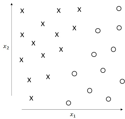
First, let’s see the following 2-class linear classification example, which has inputs of 2-dimensional vectors , and labeled values 1 (which is marked as a circle) and -1 (which is marked as a cross).

Assume that we have input data.
is the n-th input data, and is the n-th labeled value.

Note : I’m sorry, but the syntax for both and might confuse you. In this post, I use for a scalar value, and use for a vector value. (Then here.)

As you can easily see in above picture, this data can be linearly classified. Then, when we denote as weights and (scalar value) as a bias, the following equation will hold for .

when

when

Dividing these equations by , you will get the following equations. (Here .)

when

when

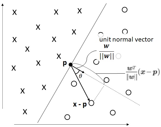
Now we pick up some position vector on boundary (see the below picture). Then this will hold .
Using this vector , the left side of above equations (1) and (2) is represented as follows.

What’s meaning geometrically ?
The value is an inner product between and . Then this value is equal to , as the following picture shows.

Note : That is, decides the direction of boundary (decision hyperplane).

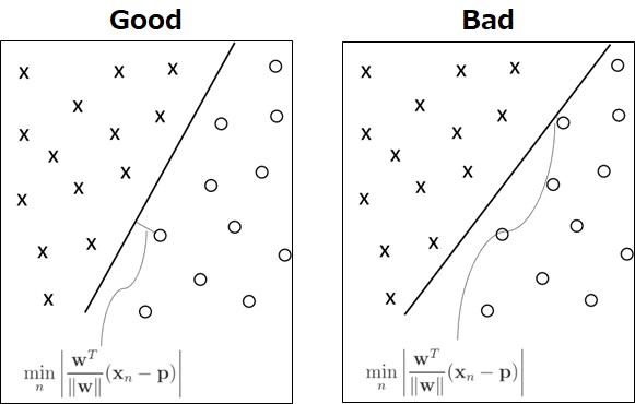
Eventually, every for is representing a distance from the boundary as a following picture. This distance is called a margin.

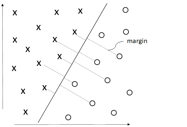
As you can see below, this margin will differ when the decision boundary has changed.

Now we assume that all input’s vectors are not on the boundary. (If there exists a vector on exact boundary, please change the boundary away from that.)
As you saw above, is a positive number, when . It’s a negative, when .
Then the equations (1) and (2) will be written as a following single equation.

We assume .
Then the above equation will be written as follows.

The decision boundary is the same as for any scalar value .
Then the above equation will also written as follows without losing generality. In the following equation, I replaced to , and to .

Now let’s consider which one is the most optimal decision boundary.

First, as you can see below (see the following picture), the decision boundary will become better, when the minimum margin is more larger.
Then you should find for obtaining the optimal decision boundary.

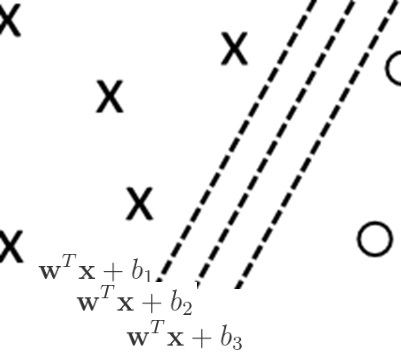
Second, when the decision boundary is obtained, this optimal doesn’t depend on .
Let’s see the following picture. If you change , only the intercept in boundary function changes and the gradient is the same.
Thus, in order to maximize margin , the optimal is given as the center between two classes. That is, if is given, the optimal (i.e, ) is determined.

Note : decides the position of boundary (decision hyperplane). Please remember that has decided the “direction” of boundary (decision hyperplane).

Here I note that there exist which satisfies in equation (3). (These definitely exist, since, if there doesn’t exist, you can get the better and then is not optimal.) We assume that these are and as follows.

Now let’s consider how the margin is give by with the condition of equation (3).
As you saw above, the margin of each is given by . Thus the minimum margin is given as :

Then, in order to maximize the class margin, you should find parameters and corresponding , which satisfies :

for all

This problem is the conditional min/max problem with inequality constraints, and we then apply the following KKT (Karush–Kuhn–Tucker) conditions with Lagrange multipliers , instead of applying Lagrange conditions. (See Wikipedia “Karush–Kuhn–Tucker conditions” for details.)

KKT condition

Find parameters , , and Lagrange multipliers to optimize the following Lagrange function , subject to the following 1 – 5. :

Note : Especillay, the condition 5 is important in KKT.

For simplicity, let me assume a single Lagrange multiplier (i.e, ).
When a Lagrange multiplier is equal to 0 (i.e, in condition 5), the condition 1 means that the optimal is the mathematical limit of the norm , and you will then find that data point doesn’t contribute to the result when .
This intuitively implies that the limit is within the range of inequality constraints , such like the left side of the following picture. (In this picture, has 2 dimensions.)

When a Lagrange multiplier is not equal to 0 (i.e, ), the condition 5 says that the optimal should be on boundary in inequality constraints , such like the right side of the following picture.
In this case, the data point is the support vector. (See below for support vector.)

Here I don’t go so far, but this problem yields to the following equivalent problems with only Lagrange multipliers by substituting and erasing .
This equivalent representation is called dual representation in mathematics.

Dual representation

Find to maximize the following :

Subject to :

• for all
• 

Note : The objective function is a quadratic function and you can then solve this problem as a Quadratic Programming (QP) problem. (You can use any generic QP solver in computer systems.)

When is obtained by the above dual representation, eventually you can get the decision boundary by the following formula. (As we saw above, can also be easily obtained, because we have .) :

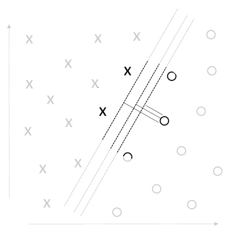
As you saw earlier, the vector (input data) which has the minimum margin is especially important for this problem. Then this vector is called a support vector in SVM.
For instance, all of the following 5 vectors are support vectors.

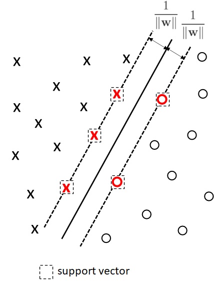
As you saw above, this problem is to get the optimal parameters by minimizing . By this mechanism, margin maximization in SVM essentially avoids overfitting by L2 regularization. (See here for L2 regularization in overfitting problems.)

Introducing Kernel Methods

In above example, we saw the idea of support vector machines (SVM) using a trivial linear classification. But, the real problem is not so simple.
From here, we enter into more practical topics step by step.

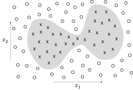
For instance, let’s see the following input vectors.
As you can easily see, this cannot be classified by any of linear decision boundary.

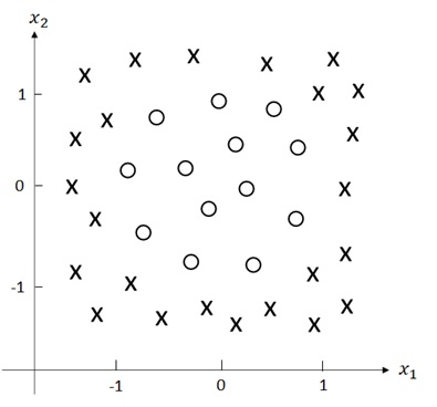
Now let me introduce kernel tricks in this section.

In order to make it classified by linear decision boundary, we assume that the above 2-dimensional vectors are mapped into more high dimensional space.
For example, let us assume that above 2-dimensional vectors are mapped into 3-dimensional vectors by the following mapping definition.

With this mapping, the data is easily classified by the 3-dimensional hyperplane, which is the grey-colored plane in the following picture.

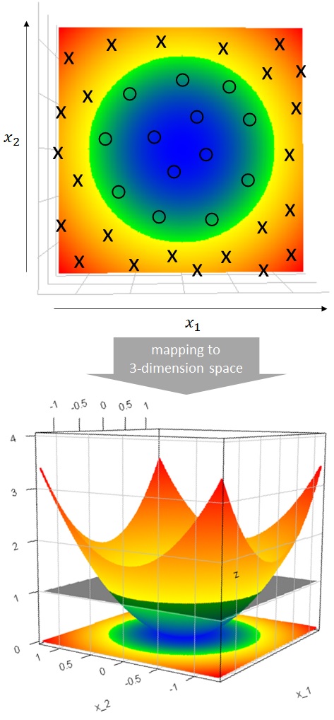
Note : As you see in above picture, the mapped coordinates are not dense. (It’s a 2-dimensional manifold embedded in 3-dimensional space.) Thus the learner with this method (with which, the inputs are mapped into high dimensional space) is sometimes called “sparse kernel machine”.

is called a basis function.
When is given, this problem (to find weight vector and bias) yields to the following dual representation. (See above section for dual representation.)

Dual representation

Find to maximize the following :

Subject to :

• for all
• 

When Lagrange multipliers, are given, you can obtain the decision boundary by the following formula. :

Now we denote as . This is called a kernel function.
Using kernel functions, we can write above (7) as follows. It’s simply given by a linear combination of the target values from the training set.

As you can easily see, above problem is all written (described) by unknown kernel without base function . The additional constraint is that should have a function , such as, . From now on, we consider this problem (mapped into high-dimensional spaces) only using the kernel .
Here I don’t describe proofs, but it’s known that many other loss functions or predictive functions (also, dual representations) in popular machine learning algorithms can also be written with kernel functions. (You can then use kernel methods in various machine learning problems.) For instance, when we apply regularized least square for regression problems with basis function : (see my previous post for linear regression by least square), it’s known that the obtained predictive function can be written as follows using some kernel function .

where is training input’s set and is corresponding label’s (target value’s) set.

Now is unknown and might be an arbitrary function, but one important constraint is “it should be kernel function”.
For instance, is a valid kernel function, since this function can be expanded as follows. :

where

It’s known that sum, product, and composition of kernel functions are also kernel functions.
However, in most cases, the way without having explicitly to construct the original basis function is used to know whether a function is a valid kernel function.

Note : In kernel methods, it’s often used a matrix called Gram matrix, which has the value on element, where is training inputs.
Gram matrix is symmetric and should be positive semidefinite, if and only if is a valid kernel function.

How should we obtain (or approximate) the appropriate kernel function in support vector machines ?
I’ll give you one of solutions for this question in the next section.

RBF Kernel – Why it’s widely used ?

In this section, we see RBF (Radial Basis Function) kernel, which has flexible representation and is mostly used in practical kernel methods.

RBF kernel is a kernel, which only depends on its norm .
Especially, the following form of kernel is called Gaussian kernel.

Note : It’s known that is a valid kernel function, if is a kernel function.
Gaussian kernel has infinite dimensionality.

In this section, I’ll show you how it fits to the real data and make you understand why this kernel (Parzen estimation) is so popular.
For simplicity, we discuss using previous linear regression at first

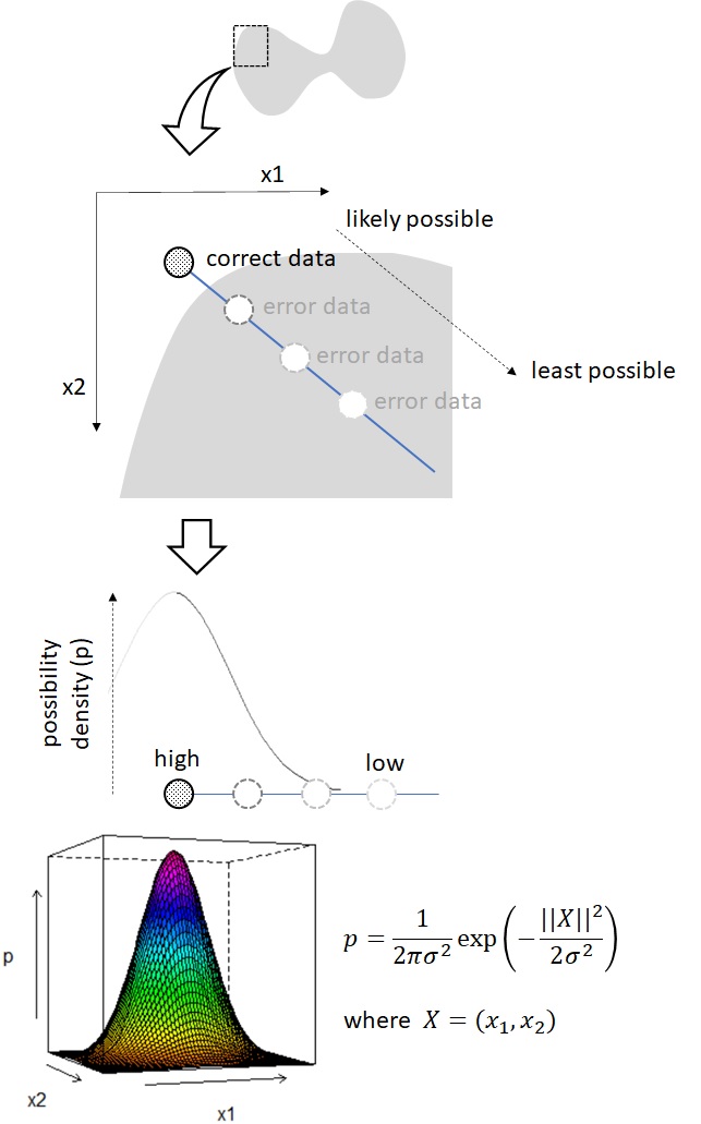
Now, to make things simple, let us assume the following binary classification of 2 dimension’s vector , and consider the possibility of errors.

As you can easily imagine, you will see the error values with large possibility when it’s near the boundary, and with less possibility when it’s far from the boundary. As you can see below, the possibility of errors will follow the 2-dimensional normal distribution (Gaussian distribution) depending on the distance (Euclidean norm) from boundary.

Note : For simplicity, here we’re assuming that two variables and are independent each other, then their covariance is equal to zero. And we also assume the standard deviation for and are both .
(i.e, the covariance matrix in Gaussian distribution is isotropic.)

On contrary, let us consider the error possibility of the following point.
As you see below, this will be affected by both upper side’s boundary and lower side’s boundary, and it will become the sum of both possibilities.

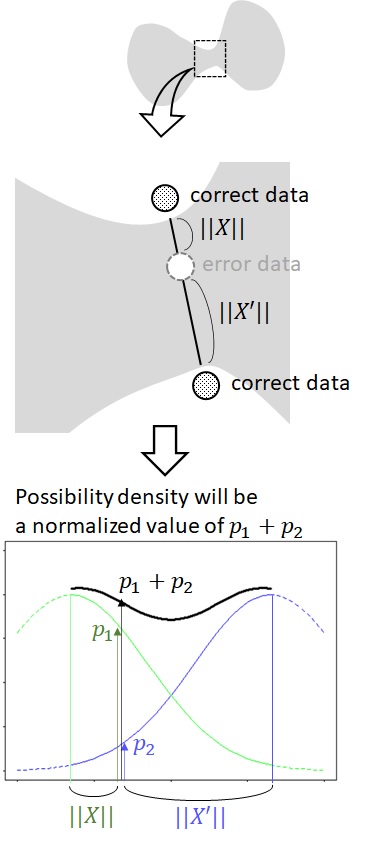
Note : If you simply add these possibilities (for upper-side and lower-side), the total possibilities will exceed 1. Thus, strictly speaking, you should normalize the sum of these possibilities.

Eventually the possibility of errors will be described as probability density distribution by the combination (sum and normalization) of normal distributions in each observed points.

In order to see this in the brief example, let us assume the following 1-dimensional sine curve and we have the following 6 observed points exact on this curve.

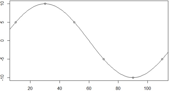
Then, by applying the following steps, we can estimate the original sine curve with these 6 points.

1. Assume normal distributions (Gaussian distributions) for each 6 observed points.
   
2. Get the weighted ratio for each distributions.
   For instance, we assume on in above picture. Then the weighted value for each elements on are :
   ,
   ,
   ,
   .
   The following picture shows the weighted plots of each distributions.
   
3. Multiply by each observed values.
   For instance, if t-value of the first observed point is 5 (see above picture of sine curve), then the effect of this first value (black-colored line) on will be equal to . (See below picture.)
   
4. Finally, sum all these values (i.e, these effects) for 6 elements on each points of x-axis.
   

Please remind that the predictive function by linear regression with basis function can be written as the linear combination between target values (t) and kernel functions. (See previous section.)
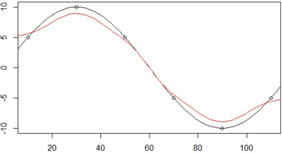
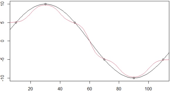
As a result, you can easily estimate original curve by Gaussian kernel using the given observed data as follows.
Gaussian kernel has rich representation and can fit to a various kind of formula.

Note : Here I showed a brief example using a simple 1-dimension sine curve, but see chapter 6.3.1 in “Pattern Recognition and Machine Learning” (Christopher M. Bishop, Microsoft) for the general steps of Nadaraya-Watson regression (kernel smoother).

in Gaussian is experimentally determined.
When is larger, the model will become more smoother. On contrary, when is smaller, the model is locally dominated by nearby observed values.

The value of standard deviation () is large

The value of standard deviation () is small

Note : Kernel density estimation (KDE) is the application for estimating the empirical probability density function (PDF) by applying this kind of Gaussian kernel smoother.
When differs extremely in each points, you can use the estimation by kNN (K nearest neighbor) method in non-parametric approach.
See “Mathematical Introduction to Regression” for the estimation application of parametric approach.

Now let’s go back to the equation (6) and (7).

In these equations, the formula of is unknown, but we can expect that these are also estimated by Gaussian kernel, and then we can get optimal Lagrange multipliers under this assumptions.
As you saw above, when is smaller in Gaussian kernel, the hyperplane will also be increasingly dominated by nearby observed data relative to the distant ones.

The kernel methods is very powerful, since it can be applied for various unknown stochastic distributions. But you should remember that the computational complexity will increase linearly by increasing the size of training data.

Note : In general, a regression function which forms a linear combination of kernel by the training set and target values, , is called a linear smoother.
Here we got this form by intuitive thinking, but you can obtain the equivalent regression result by Bayesian inference (algebraic calculation) for a linear basis function.

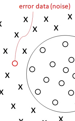
Overlapping Class Distributions

Until now, we assumed that all data is exactly separated by support vector machines (i.e, hard-margin SVM). However, there’ll also be observed errors (noise) in practical SVM.
Here I show you soft-margin SVMs (such as, C-SVM and ν-SVM) which evaluate these losses.

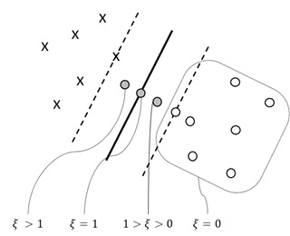
First of all, I introduce new variable (called slack variables) which satisfies :

for any

subjects to :

• , when it exceeds decision boundary.
• , when it’s on decision boundary.
• , when it’s between decision boundary and margin.
• , others (when it’s correctly outside of margin, including support vectors.)

In the previous problems (without considering losses), we found to satisfy conditions.
Instead, in this problem, we find the parameters to minimize the following equation.

Note : The above loss formula is also written by :

where

The part is sometimes called hinge loss. (The name is because of the shape of the function .)

Here the constant is a penalty for loss, and it’s determined experimentally by using such as cross-validation. (Later I’ll show you how affects the model.)

This is called C-SVM (C-support vector machine), and it’s also solved by dual representation with Lagrange multipliers. (I don’t describe this mathematical solution in this post.)

Let’s see another soft-margin SVM, called ν-SVM (ν-support vector machine).
In the previous C-SVM, if the number of inputs, , increases, the penalty will also linearly increase. That is, there will be the bias depending on .

In ν-SVM, this bias is suppressed by using .
ν-SV classifier is defined as :

• Find to minimize
• Subject to : for any

With condition , the margin becomes . Then if is smaller, the loss will also be smaller. Eventually this classifier might pick up so small margin and will cause overfitting. (Then will become so large.)
To prevent this unexpected learning, the term is introduced in this classifier.
Same like in C-SVM, is also determined experimentally.

Note : In this post, we’re discussing 2-class problems. However, even when only one class of data (i.e, only true data) is given, you can also obtain the optimal shpere by optimizing (i.e, the distance from boundary). By this approach, this trained model can then detect outside of the boundary – i.e, outlier or anomaly – by only using true data (inlier data) in training.
This learner is useful, because it is usually difficult for you to collect sufficient error (outlier) data. This learner is called one-class SVM. (I note that there exists another type of one-class SVM, but I don’t go details so far in this post.)
See here for training and prediction by one-class SVM in Python.

Let’s consider how this affects to the model.

To see this, now I show you corresponding KKT condition for this ν-SVM as follows.

KKT condition

1.
2.
3.
4.
5.
6.
7.
8.

From condition 3 and 6, we get .
When we denote the number of support vectors as , the number of is at most from condition 7.
Then, from condition 4, we get :

It means that the ratio of support vectors is equal or larger than .

On contrary, the vector which satisfies (i.e, the noise vector) is called bounded support vector, and we denote the number of bounded support vectors as .

From condition 8, the bounded support vector has . From condition 3, it means .
Then we get :

It means that the ratio of bounded support vectors is equal or smaller than . (This is the reason of the name of “bounded support vector”.)

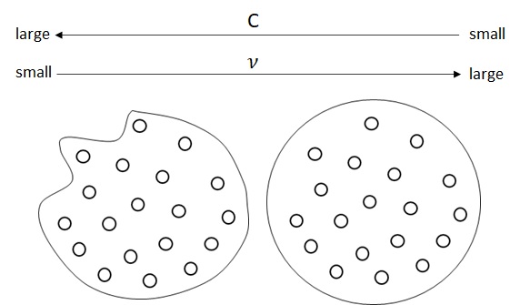
The following picture shows how (or in C-SVM) intuitively affects model. When increases (or decreases), both support vectors and bounded support vectors will tend to increase.

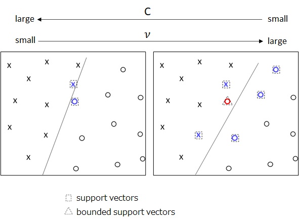
With high dimensional mappings, this parameter will affect the trained model, such as the following image.
In general, when is smaller, the model complexity will become higher, and it might become rich enough to represent more complicated problems. However, this might also cause overfitting. (On contrary, when get larger, the model becomes more generalized.)
This parameter should be experimentally determined to fit the real problems, considering these trade-off.

Note : For details about overfitting, see my early post “Mathematical Understanding of Overfitting in Machine Learning“.

For training support vector machines in real computing, the analytical algorithm (such as, sequential minimal optimization) will be applied to fit in memory and scalability.

In this post, we have observed mathematics fundamentals behind SVMs and kernel tricks.
This idea of margin maximization gives you optimal solutions for high dimensional separation, and the idea is then also applied in a variety of other ML tasks – such as, inverse reinforcement learning (IRL), etc.

Reference :

“Pattern Recognition and Machine Learning” (Christopher M. Bishop, Microsoft), Chapter 6 and 7