(Download source code from here.)

In order to tackle a variety of problems with quantum computing, it’s important to know and make use of quantum algorithms.
In this post and series, I’ll introduce several key quantum algorithms and these implementation with Q# programming.

• Programming Quantum Algorithm for Beginners (Bernstein-Vazirani algorithm)
• Programming Quantum Search (Grover’s Algorithm)
• Programming Quantum Phase Estimation
• Programming Quantum Arithmetic (Adder, Multiplier, and Exponentiation)
• Programming Quantum Period Finding (Shor’s Algorithm)

First, in this post, I’ll show you primitive programming example with Bernstein-Vazirani algorithm for your very beginning and introduction.
It has no practical use, but it can be your first example (a getting-started example) of a quantum algorithm.

By installing local simulator (such as – Quantum Development Kit, shortly QDK), you can run Q# code in your local computer, without needing real quantum devices. (See here for installation.)
It’ll be a good place for prototyping quantum algorithms quickly and free of cost. In order to deepen your understanding, let’s try running the following code on your local machine.

Bernstein-Vazirani algorithm

First, let’s start with classic (non-quantum) fashion.

Here we suppose is given and unknown.
Now we consider the following transformation , in which is a classical logic gate.

where and

Note : In the paper, is used for , but here we have omitted without losing generality.

In order to find unknown values , you would check the following values .
(For simplification, here I fix .)

If there’s 100 unknown variables, you will need 100 trials.
That is, it will need polynomial frequency of computation to solve this problem in classical algorithms.

In quantum fashion, you can find with only one computation (which includes 3 steps) with Bernstein-Vazirani algorithm.

The idea of this algorithm is based on the properties for generated by Hadamard gate .
Hadamard gate (see here) is a special transformation and widely used for various algorithms, because this can generate the uniform states for all qubits such that :

As you can see below, when you apply Hadamard twice, it turns into the original position. (Here I show the result for , but this holds for any dimensional .)
and have the same outcome for quantum measurements and the difference won’t be observed for humans, but you can find the difference by applying Hadamard again.

Note : See here for the meaning of (Hadamard for a single qubit) with Bloch sphere representation.
If ( and are real numbers and ), the transformation is the reflection across the line in 2-dimension space (in which, -axis and -axis are basis).

These properties lead to the following Bernstein-Vazirani quantum algorithm by also applying Hadamard operation twice. :

Bernstein-Vazirani algorithm

1. Suppose we start with the following n + 1 qubits :
   ,
   
   Here you can get and by :
   
   
   where is Hadamard operation.
2. I denote by .
   Apply transformation where is equivalent to the classical bitwise XOR. ( is then reversible and unitary.)
   In quantum fashion, can be implemented (substituted) by quantum CNOT operation. (Later I’ll show you details.)
3. Apply Hadamard gate again for and measure .
   The result will then be our expecting .

Unlike classical methods, you don’t need to check all , , , and .

If you are new to quantum algorithms, you might think that it’s curious because is not applied for any transformation in this algorithm. But quantum state of is changed by applying the quantum entanglement (CNOT) in #2. (See here for entanglement.)
Here I don’t go deep dive, but it’s known that when . (In this equation, means that positive / negative turns into negative / positive, when .)
Thus this method is sometimes called phase kickback.

Note : See the lecture “Lecture 4: Elementary Quantum Algorithms” (CS 880 – Quantum Information Processing in University of Wisconsin-Madison) for phase kickback method and Bernstein-Vazirani algorithm.

Let’s say, we assume

and as follows.

By applying for in these assumptions, it will then become the following result, because it satisfies at .

By applying Hadamard again, these state’s change will be reflected back to and you can then observe the difference.

Note : See here for algebraic computation in these assumptions.

Now we’ll implement this simple algorithm using Q# code below.

Q# Programming for Bernstein-Vazirani algorithm

In this post and series, I’ll run quantum program on local simulator. Before starting, please install and setup Quantum Development Kit (QDK) in your local computer. (See here.)
Here I’ll build quantum logic with Q# in the backend, and invoke this procedure from Python code in the frontend. All inputs / outputs (facing to users) are handled by Python and these values are passed into the Q# code.

Note : You can also use C# (.NET) for the frontend, instead of Python.

First we define unknown in Python as follows. (To simplify example, here I fix and .)
For instance, if parity = 11, it means 1011 (2) and .

Initialize values on Python

import randomn = 4parity = random.randint(0, 1 << n - 1)# pass "parity" to Q# code... (run quantum simulator)...

From here, it all runs on quantum simulator, Q#.

I assume that above “parity” is passed into Q# code as follows.
The following “pattern” (which is in Q# code) will then become [true, false, true, true], when parity = 11 (i.e, 1011 (2)).

Runs on Quantum Simulator (Q#)

let pattern = IntAsBoolArray(parity, n);

First we initialize and in Q#.
In this code, qubits[i] where i=0 … n-1 (which has n elements) is , and last qubits[n] is . By applying Pauli-X for , it will change the initial state to . (See here for Pauli-X (NOT) gate.)

// all n+1 qubits are initialized as |0〉use qubits = Qubit[n + 1] {  // set only last qubits[n] as |1〉  X(qubits[n]);  ...

Note : For debugging, you can use Q# function Microsoft.Quantum.Diagnostics.DumpMachine() to print the state of the quantum computer (simulator).

By applying Hadamard gate for all qubits, then becomes , and becomes . (See above #1 in Bernstein-Vazirani algorithm.)

// set qubits[i] = |+〉 (i=0 ... n-1) and qubits[n] = |-〉ApplyToEach(H, qubits);

Next we’ll define unitary transformation #2 (in Bernstein-Vazirani algorithm) as follows.

Note that the following variable “qs” takes the previous “qubits“, in which qubits[i] (i=0 … n-1) represents and qubits[n] represents .

By applying Controlled X(a, b) (Controlled-X or CNOT gate), “a” is used as control bit and X (= NOT gate) is applied to target “b”. As you can easily see, this operation is equivalent with classical XOR and it will then represent in #2. (Note that quantum state doesn’t have the logical bitwise operation. For implementation of classical logic gate in quantum computing, see “Lecture 2: From Classical to Quantum Model of Computation“.)
By the beauty of Q# abstraction, this for-loop iterations (also ApplyToEach() operation above) is equivalent to the multi-qubit operations (where is some single operation with controlled and adjoint).
As a result, this operation will create a circuit for unitary transformation .

Note : “Unit” means “no result” in Q#. (It’s like “void” in C#.)

operation ParityOperationImpl (pattern : Bool[], qs : Qubit[]) : Unit {  let n = Length(pattern);  for idx in 0 .. n - 1 {if (pattern[idx]) {  Controlled X([qs[idx]], qs[n]);}  }}function ParityOperation (pattern : Bool[]) : (Qubit[] => Unit) {  return ParityOperationImpl(pattern, _);}

Now we apply this unitary transformation for above “qubits” ( and ).

let Uf = ParityOperation(pattern);Uf(qubits);

Finally we apply Hadamard again for (i.e, qubits[i] i=0 … n-1) and measure these qubits for getting result.
When you compare this result with previous “parity“, you will find these ( where ) are exactly same values.

// apply Hadamard again except last qubitApplyToEach(H, qubits[0 .. n - 1]);// measure and reset qubitlet resultArray = ForEach(MResetZ, qubits[0 .. n - 1]);let resultBool = ResultArrayAsBoolArray(resultArray);let resultInt = BoolArrayAsInt(resultBool);

The completed example (entire code) is below. :
(You can download and run source code from here.)

Q#

open Microsoft.Quantum.Intrinsic;open Microsoft.Quantum.Canon;open Microsoft.Quantum.Measurement;open Microsoft.Quantum.Arrays;open Microsoft.Quantum.Convert;operation BernsteinVaziraniTestCase (n : Int, patternInt : Int) : Int {  let pattern = IntAsBoolArray(patternInt, n);  use qubits = Qubit[n + 1] { // all n+1 qubits are initialized as |0〉// set only last qubits[n] as |1〉X(qubits[n]);// set qubits[i] = |+〉 (i=0 ... n-1) and qubits[n] = |-〉ApplyToEach(H, qubits);// apply unitary transformation for qubitslet Uf = ParityOperation(pattern);Uf(qubits);// apply Hadamard againApplyToEach(H, qubits[0 .. n - 1]);// measure and reset qubitlet resultArray = ForEach(MResetZ, qubits[0 .. n - 1]);let resultBool = ResultArrayAsBoolArray(resultArray);let resultInt = BoolArrayAsInt(resultBool);// reset last qubitReset(qubits[n]);return resultInt;  }}operation ParityOperationImpl (pattern : Bool[], qs : Qubit[]) : Unit {  let n = Length(pattern);  for idx in 0 .. n - 1 {if (pattern[idx]) {  Controlled X([qs[idx]], qs[n]);}  }}  function ParityOperation (pattern : Bool[]) : (Qubit[] => Unit) {  return ParityOperationImpl(pattern, _);}

Python (Use Python or .NET)

import randomn = 4parity = random.randint(0, 1 << n - 1)measuredParity = BernsteinVaziraniTestCase.simulate(n=n, patternInt=parity)print("Actual Parity is {}".format(parity))print("Measured Parity is {}".format(measuredParity))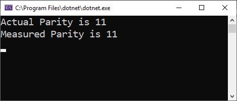

Note : Deutsch-Jozsa algorithm is also a famous algorithm based on phase kickback technique, and you can see example in official GitHub repository (Microsoft/Quantum).

Reference : Quantum Computing Introduction (Physics & Maths)